Lecture 1: Algorithms & Analysis

Algorithm

A clearly specified set of instructions to be followed to solve a specific problem
- Adding two n-digit numbers
- Sorting a list of n names
- Finding one student’s name among N students
This N is important
- The number of items we are dealing with
- What happens as N grows very large
Sequential search → O(N) time
Binary search → O(log N) time, but the list must be sorted
2³² is 4 billion → only 32 comparisons to search all 8 billion people if you cut in half each time

Important Questions About Algorithms

Is it correct?
How much extra memory does it require? → memory complexity → see how memory is physically organized in ICS 51
How long does it take? → time complexity

The analysis of these two questions is critical to algorithm selection

T(N)

The time required for an algorithm to run on input of size N
Simple instructions → +1 operation (+, −, ·, /, …)
Loops → sum of nested instructions times the number of loop iterations
Function calls → T(N) of the called function
If/else → maximum of either branch plus the cost of the condition
- Only one branch executes, so take the worst case PLUS the additional check of the condition (which can involve multiple checks)

How to Report T(N)

State the actual polynomial and say it is equal to the following
Count the number of run-time instructions

Example: Summing 1 to N

int sum( int N )
{  
    int result = 0; // 1
    for( int i=1;   // 1
          i <= N; ++i )     // 2        LOOP N TIMES -> N * ( 2 + 2 = 4)
            result = result + i;  // 2
    return result;  // 1
}

T(N) = 4N + 3

int sum( int N )
{     
    return N * ( N + 1 ) / 2;
}

T(N) = 4
The return adds 1 plus all the expressions

Example: Strange Sum

int strangeSum( int A[N] )
{
        int total = 0; //1
        for(int i=0; //1
         i < N; ++i ) // n-1, 1
            total = total + A[i-1] * A[i]; //4
        return total; //1
}

Array indexing → cost of the index plus 1 (same rule as return)
T(N) = 8N + 3
- Outside of loop there are 3 operations
- The 8 inner operations happen from 0 to N times → total of N times

Example: Bubble Sort

void swap( int & a, int & b )  // T(N) = 3
{
    int t = a; a = b; b = t;
}
 
void bubbleSort( int A[N] )  // A tricky one...
{
  for ( int a = 0; a < N; a++ ) // RUNS N times
      for ( int b = N - 1; b > a; b-- ) // sum of all N integers with the combination of 2 loops
          if ( A[b-1] > A[b] )    // condition is 4  // IF is 4 + max(6,0) = 10
              swap( A[b-1], A[b] ); // then part is 6 (the accessing is 3 plus the call of the function)
}

N · (N − 1) / 2 is the closed form for the sum of N integers
T(N) = 10 · (N · (N + 1)) / 2 →
5 · (N² + N) →
5N² + 5N + 1 → final form

GitCodings

// What is T(N) of strlen(), if N is the length of s?
int strlen( char *s ) { 
    int len = 0;
     for ( int i = 0; s[i] != 0; ++i )
          ++len;
     return len;
}
 
// My Guess: T(N) = 4N + 3
// Right Answer: T(N) = 4N + 3

int strchr( char c, char *s ) // V1
{
       for ( int i=0; i < strlen(s); ++i )
               if ( s[i] == c )
                      return i;
       return -1;
} 
// My Guess: T(N) = 2(4N + 3) + 2

The strlen is 4N + 3 plus 2 for the other 2 operations in the for loop
- N · (4N + 5 + 3) for the if statement, then plus 2 for the outside of the loop
- T(N) = 4N² + 8N + 2

int strchr( char c, char *s )  // V2
{
       int len = strlen(s);
       for ( int i=0; i < len; ++i )
               if ( s[i] == c )
                      return i;
       return -1;
}

T(N) =
- First: initialize len plus strlen → 4N + 3 + 1
- Loop runs N times with 5 operations inside
- Return → +2
4N + 4
5N + 2
T(N) = 9N + 6 → correct answer!

// What is T(N) of strchr(), if N is the length of s?
int strchr( char c, char *s )  // V3
{
       for ( int i=0; s[i] != '\0'; ++i )
               if ( s[i] == c )
                      return i;
       return -1;
}

1 for the initialization
6N + 2 → confident
Real answer is: that I am a dawg

Asymptotic Analysis

As N gets larger, what is the performance hit?
When you multiply by large numbers, things grow rapidly
Best Case
Worst Case
Expected Case (Middle)

Big-O Notation

As N gets large, the lower-order terms are negligible
We care most about the highest-order term
T(N) = 4N² + 6N + 40
T(N) = 2N⁴ + 1000N² + 30N + 2000
Big-O (pronounced “big oh”)
- T(N) = O(f(N)) if there are positive constants c and n₀ such that T(N) ≤ c · f(N) when N ≥ n₀
- Don’t care about low orders of N
- Find what it is bounded by
Big-O → upper bound (the closest function that bounds it from above)
Omega → lower bound
Theta → tightly bound (strictly exactly there)

Typical Growth Rates

Function	Name
C	constant
log N	logarithmic
N	linear
N log N	log-linear
N²	quadratic
2ᴺ	exponential
N!	factorial

2³² is 4 billion
2³³ is 8 billion
10¹⁰⁰ is about 70!

Ranking of Big-O (Slowest Growth to Fastest)

O(1)
O(log N)
O(N log N)
O(N²)
O(2ᴺ)
O(N!)

Reporting Big-O → just say “Big-O of N²” and that’s all

Activity

T(N) = 10N⁴ + 2N² log N − N³ → O(N⁴)
T(N) = log₂ N + N log N + N² → O(N²)
T(N) = Nᴺ + N! → O(Nᴺ)
T(N) = 2^(N/2) + 3N log N → O(2ᴺ)

Lecture 2: Unordered Lists

Unordered Lists

Lists may be
- Unordered
- Ordered
- Sorted
Typical operations
- insert, find, remove, length, print
Lists may be implemented as
- An array list (within an array) → memory is a linear array at the hardware level
- A linked list (using nodes with links/pointers)
Always consider time complexities → Big-O from Lecture 1

Unordered List: Implemented as Array

What data members do we need?
- The array
- Capacity → physical size (possible), don’t exceed capacity
- Current size → logical size (actual size)
Think about each operation (algorithm)
1. insert
2. find
3. remove
How can each be implemented efficiently given the requirements? (Unordered)

Unordered Array List

// Example is a List of char
 
class UnorderedArrayList {
    char * buf;  // an array of List Elements (char)
    int capacity;
    int size;
public:
    UnorderedArrayList(int cap)
        :buf{new char[cap]}, capacity{cap}, size{0}
    { }

Adding to Front vs Adding to End

size is the index of the next available slot
Adding to the front causes you to shift all existing elements over

Efficiency on Removal

Removal can be done by replacing with the last element and decrementing size
Don’t have to null out values → they are effectively gone

Insert

void error(string msg) {
    cerr << "WTH: Error: Who wrote this code" << msg << endl;
}
 
// adds 'c' where it belongs in this list 
void insert(char c) {
 
    // This was added post checking the first normal case
    if (is_full()) {error("UAList::insert() into full list");}
       
    buf[size++] = c;
    // Notice the post-increment: it uses the original value and THEN increments 
}

Write the first normal case
Add error checking (beginning in this case)

Find

// returns index of 'c' 
int find(char c) { 
     for (int i = 0; i < size; ++i) {
       if (buf[i] == c) {return i;}
     }
   error("Not found");
}

Remove

// removes first occurrence of c
 
int remove(char c) { 
    for (int i = find(c); i < size - 1; i++) {
        arr[i] = arr[i + 1];
    }
    --size;
}

Not sure about this one → figure it out later

Measuring Performance

Divide the data into partitions (e.g., 10)
Measure on first partition
- Then first and second
- Then first, second, third, etc.
Plot N vs T(N)
Graph shows the time complexity of the function
Must be careful to time only the work of interest
- start() and stop() timer around the work
We measure insert_all(), find_all(), remove_all() → why?
- There is jitter (variation) in data, and under large data sets it’s more visible

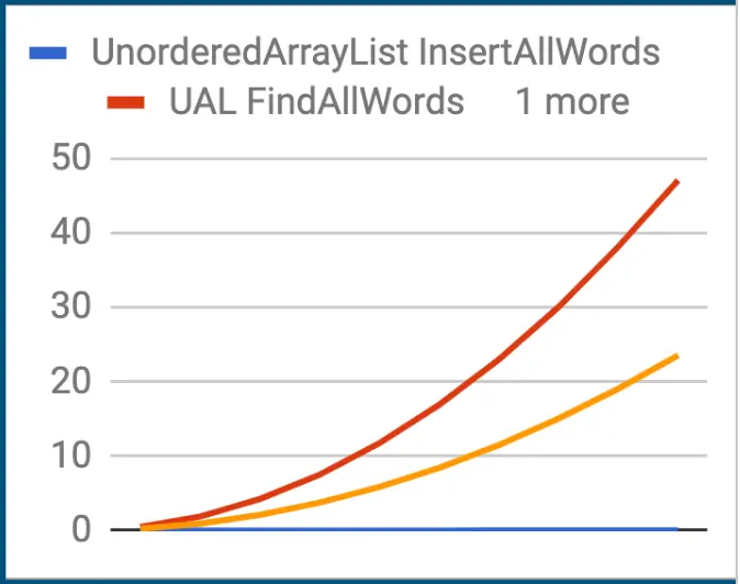
No zigzag line → should be a smooth curve
45,392 words is specific to our word set
- Start with 1/10th of the data, then 2/10ths, etc.

Framework vs Library

A library works within your software. Your software works inside a framework.
To build a framework you need virtual functions and abstract classes
Write the measurement code only once → that’s the framework’s job

Architecture vs Framework (Aside)

Architecture → high-level, abstract plan for a system defining major components and their interactions
Framework → concrete, reusable set of code and libraries that helps implement an application within the boundaries set by the architecture

Unordered List Implemented as Linked List

Use a helper class ListNode
- Two data members:
  - data (string in this case)
  - next (pointer to next ListNode)
Useful to write helper methods
- Allows more re-use of helper functions
- Allows recursion
- Simplifies non-static list methods
Think about each operation:
- insert → insert at head (unordered, so position doesn’t matter)
- find
- remove

Singly Linked List Node

// ListNode helper class
struct ListNode {
    char data;
    ListNode * next;
};
 
ListNode * p = nullptr;          // the empty list
p = new ListNode{d, p};          // adds d onto front of p
// Uses curly-brace (aggregate) initialization, not parens
// Data members must all be public for this to work

Linked List insert()

class UnorderedLinkedList {
    struct ListNode {
        char data;
        ListNode * next;
    };
    ListNode * head;
 
public:
    UnorderedLinkedList() : head{nullptr} { }
 
    void insert(char c) {
        head = new ListNode{c, head};
    }
};

Linked List find()

class UnorderedLinkedList {
    // private static helper — searches from node L
    static ListNode * find(char c, ListNode * L) {
        for (ListNode * p = L; p != nullptr; p = p->next) {
            if (p->data == c)
                return p;
        }
        return nullptr;
    }
 
public:
    char & find(char c) {
        ListNode * p = find(c, head);
        if (p != nullptr)
            return p->data;
        // else: do whatever is appropriate
        // e.g., could add c to head of list, then return head->data
    }
};

Linked List length()

class UnorderedLinkedList {
    static int length(ListNode * L) {
        int count = 0;
        for (ListNode * p = L; p != nullptr; p = p->next)
            ++count;
        return count;
    }
    ListNode * head;
 
public:
    int size() {
        return length(head);
    }
};

Linked List remove()

class UnorderedLinkedList {
    static ListNode * remove(char c, ListNode * L) {
        // implementation left as exercise
    }
    ListNode * head;
 
public:
    void remove(char c) {
        head = ListNode::remove(c, head);
    }
};

Lecture 3: Sorted Lists & Binary Search

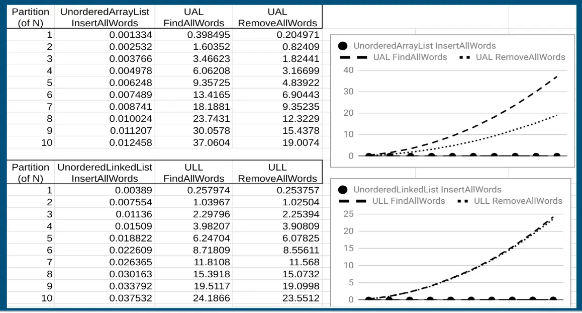
Benchmarking Unordered Lists — Theory vs. Reality

The measured times don’t match the predicted Big-O complexities — why?
Array List anomalies:
- Insert all → predicted O(1) per insert, measured O(N) total — makes sense, we’re calling O(1) insert N times
  - Inserting at the end in the same order as the file → truly O(1) each
- Find all words → predicted O(N) per find, but measured ~100× slower than insert
  - Calling O(N) find N times → O(N²) total
- Remove all words → should also be O(N²) like find-all, but measured at roughly half the time of find-all
  - Why half? The “swap-to-back” removal trick: find the word, swap it with the last element, decrement size → the removal itself is O(1)
  - Each successive removal shrinks the array, so on average you’re searching through N/2 elements → total work ≈ N²/2
  - First removals are fast (element might be near the front or the array is large but you get lucky), later removals search a smaller array but from the start
Linked List:
- Insert all → O(1) per insert (prepend to head), O(N) total
- Find all words → O(N) per find × N words → O(N²) total
- Remove all words → O(N) per remove × N words → O(N²) total
Why does the array’s remove-all take half the time but the linked list’s doesn’t?
- Array remove uses the swap-to-back trick → each removal is O(1) after finding, and the shrinking array means average search length is N/2
- Linked list remove has no such shortcut — you traverse to find the node, then unlink it (O(1) unlink, but still O(N) traversal each time), and unlinking doesn’t reduce traversal time the same way because you still walk from the head every time
- Both end up O(N²), but the array version has a constant factor of ~½
Aside: What does N · log N look like? → just a tiny bit more than O(N) — nearly linear

Other List Types

We’ve studied unordered lists, but there are others:
Circular lists → e.g., repeat playlist in a music player — last node points back to first
Doubly Linked List → e.g., std::list in C++
- O(1) insert(), O(1) remove() (given a pointer to the node), O(N) find()
Ordered lists → items retained in insertion order
- Operations: insert, find, remove
- e.g., std::string (characters in order of insertion)
Sorted lists → items retained in sorted order
- e.g., student roster, phone book
Performance tradeoff aside:
- find is the most frequently called operation in practice
- Unordered lists → insert is the fast one (O(1) prepend/append)
- Sorted lists → find is faster (binary search possible on arrays)

Sorted Lists

Similar to unordered lists, but items are maintained in sorted order
- Order may be ascending or descending
- Approach: insert incrementally in the right spot (not “dump everything in, then sort” — that’s eager sorting and it’s wasteful)
- e.g., student roster, phone book, book index
Typical operations: insert, find, remove, length, print
May be implemented as:
- Array list:
  - find → O(log N) using binary search
  - insert → O(log N) to find position + O(N) to shift elements right → O(N) total
  - remove → O(log N) to find + O(N) to shift elements left → O(N) total
- Linked list:
  - find → O(N) linear scan (can’t do binary search — no random access)
  - insert → O(N) to walk to the right spot + O(1) to link → O(N) total
  - remove → O(N) to find + O(1) to unlink → O(N) total
How to keep it sorted? → Incrementally — insert each new element in its correct position

Quick recall: 2³² = ~4 billion, 2³³ = ~8 billion

Sorted Array List — Class Definition

class SortedArrayList {
    char * buf;
    int capacity;
    int size;
public:
    SortedArrayList(int cap)
        : buf{new char[cap]}, capacity{cap}, size{0}
    { }
};

Member initializer list order: the initialization happens in order of declaration of data members, NOT the order they appear in the initializer list
- Here the declaration order is: buf, capacity, size — so they initialize in that order
- This is correct and safe here because buf’s initialization (new char[cap]) uses the constructor parameter cap, not the member capacity
- If buf’s init depended on capacity being set first, we’d have a bug since buf is declared (and thus initialized) before capacity

Binary Search (Array)

// Returns the index where ‘c’ IS or WHERE IT WOULD GO if inserted
// This lets us reuse binary_search for find, insert, AND remove
int binary_search(char c, char A[], int low, int high) {
    while (low <= high) {
        int mid = low + (high - low) / 2;  // avoid overflow vs (low+high)/2
        if (A[mid] == c)
            return mid;          // found it
        else if (A[mid] < c)
            low = mid + 1;       // search right half
        else
            high = mid - 1;      // search left half
    }
    return low;  // not found — low is the insertion point
}

Returns the insertion point — the index where c would go to maintain sorted order
If the element exists, it returns its index; if not, it returns where it should be
Complexity: O(log N) — halving the search space each iteration

Binary Search on a Linked List?

You technically can’t do efficient binary search on a linked list — there’s no O(1) random access
To reach the “middle” node you’d have to walk N/2 links → O(N)
Doing that recursively still ends up O(N) total (N/2 + N/4 + N/8 + … ≈ N)
So linked list find remains O(N) — binary search doesn’t help here
This is the key advantage of sorted array lists over sorted linked lists

Using binary_search as a Helper

binary_search() is the core helper — find, insert, and remove all use it
find(c): call binary_search(c, buf, 0, size-1) → get index i → check if buf[i] == c → O(log N)
insert(c): call binary_search to get insertion point → shift elements right → place c → O(N) due to shifting
remove(c): call binary_search to find it → shift elements left → O(N) due to shifting
Not all O(N) are equal — the constant factor matters when complexities are the same

Sorted Array List: find()

// Uses binary_search helper — O(log N)
bool find(char c) {
    int i = binary_search(c, buf, 0, size - 1);
    return (i < size && buf[i] == c);
}

copy_down — Shifting Elements Left (for remove)

// Array version — shift elements left to fill the gap at index ‘pos’
void copy_down(char A[], int pos, int size) {
    for (int i = pos; i < size - 1; ++i)
        A[i] = A[i + 1];
}

Used in remove(): find the element via binary search, then shift everything after it one position left
O(N) in the worst case (removing the first element)

copy_up — Shifting Elements Right (for insert)

// Array version — shift elements right to make room at index ‘pos’
void copy_up(char A[], int pos, int size) {
    for (int i = size; i > pos; --i)
        A[i] = A[i - 1];
}

Used in insert(): binary search for the insertion point, shift everything right, then place the new element
O(N) in the worst case (inserting at position 0)

Sorted Array List: insert() and remove()

void insert(char c) {
    int pos = binary_search(c, buf, 0, size - 1);
    copy_up(buf, pos, size);  // make room
    buf[pos] = c;
    ++size;
}
 
void remove(char c) {
    int pos = binary_search(c, buf, 0, size - 1);
    if (pos < size && buf[pos] == c) {
        copy_down(buf, pos, size);
        --size;
    }
}

Unordered List: equal()

// Two unordered lists are equal if they have the same elements (in the same order for this version)
bool equal(const UnorderedArrayList & other) const {
    if (size != other.size) return false;
    for (int i = 0; i < size; ++i) {
        if (buf[i] != other.buf[i]) return false;
    }
    return true;
}

Testing Aside

Nominal testing → test normal/expected inputs (the “happy path”)
Boundary conditions → test edge cases:
- Front and end of structure
- Empty string and single-character string in reverse_string
- Empty list, single-element list, duplicate elements

Lecture 4: Linked Lists

Sorted Linked List: Find

If the list is sorted and we pass the value we’re searching for → stop early
- No point continuing once curr->data > c

Writing Methods Recursively

Watch out for large N on an O(n) recursion → blows the stack
Prefer iteration when depth can grow with input size

Pointers

Pointers are cheap
Common pattern for traversal/mutation → prev, curr, next

Sorted Linked List: insert()

// return list with c added in the correct (sorted) spot
static ListNode * ListNode::insert(char c, ListNode * L) {
    ListNode * node = new ListNode(c);
 
    // empty list or insert at front
    if (L == nullptr || c <= L->data) {
        node->next = L;
        return node;
    }
 
    // find the node after which c belongs
    ListNode * curr = L;
    while (curr->next != nullptr && curr->next->data < c) {
        curr = curr->next;
    }
    node->next = curr->next;
    curr->next = node;
    return L;
}

Sorted Linked List: find()

// return pointer to node containing c, nullptr otherwise
// sequential search down L, stop when c >= L->data (sorted list)
static ListNode * ListNode::find(char c, ListNode * L) {
    while (L != nullptr && L->data < c) {
        L = L->next;
    }
    if (L != nullptr && L->data == c) return L;
    return nullptr;
}

Sorted Linked List: remove()

// return list with c removed
static ListNode * ListNode::remove(char c, ListNode * L) {
    if (L == nullptr) return nullptr;
 
    // case: removing the first node
    if (L->data == c) {
        ListNode * rest = L->next;
        delete L;
        return rest;
    }
 
    // walk with prev/curr, stop at match or past-it (sorted)
    ListNode * prev = L;
    ListNode * curr = L->next;
    while (curr != nullptr && curr->data < c) {
        prev = curr;
        curr = curr->next;
    }
    if (curr != nullptr && curr->data == c) {
        prev->next = curr->next;
        delete curr;
    }
    return L;
}

Three cases to test:
1. Maintain a prev pointer
2. Test on a middle node
3. Test on the first node
4. Test on the last node

Recursive Linked List remove()

// not suitable for O(N), but fun to write
static ListNode * ListNode::remove(char c, ListNode * L) {
    if (L == nullptr)
        return nullptr;
    else if (L->info == c) {
        ListNode * ret = remove(c, L->next); // remove all? or first?
        delete L;
        return ret;
    }
    else {
        L->next = remove(c, L->next);
        return L;
    }
}

SLL Remove Challenge

Given pointer P to node containing item V → remove V in O(1) time
Others may have pointer to same node P points to
How can you do this?
Hint: data is not tied to the ListNode

SLL Remove Clever Trick

// data is not tied to the ListNode!!!
static void remove(ListNode * P) {
    // P is pointing to node with value to remove
    ListNode * to_die = P->next;   // gonna delete next node instead
    P->info = P->next->info;       // copy data & next from P->next
    P->next = P->next->next;
    delete to_die;                 // delete the next node
}
// does not handle deleting the last element of the list
// works for insert() V before value at P too!

Bubble Sort

void bubble_sort(int A[], int N) {
    int i, j;
    for (i = 0; i < N; ++i)
        for (j = 0; j < N - i; ++j)
            if (A[j] > A[j+1])
                swap(A[j], A[j+1]);
}

Lecture 5: Stacks & Queues

Overview

Containers for elements → element type is a template parameter
Elements are inserted and removed → the difference is the order they come out
Useful for many algorithms
- Browser back button
- Line of customers waiting to check out
- Print requests
- Matching parentheses
- etc. (toooo many options)

Pre-Test Self-Check

What is the insert/remove behavior of a queue?
- FIFO → First-In-First-Out, elements come out in the same order they went in
What are the standard operations on a queue?
- enqueue, dequeue, front/peek, is_empty, is_full
How can you implement a queue using an array (with an initial capacity) so each operation is O(1)?
- Circular buffer with front and rear indices → enqueue at rear, dequeue from front, both O(1)
How can you implement a queue using a singly linked list so each operation is O(1)?
- Keep both head and tail pointers → insert at tail, pop at head
What errors are likely with a queue?
- dequeue() or peek() on an empty queue
- enqueue() on a full queue

Queues

Works like the check-out line at the grocery store → FIFO
Applications:
- Print queue on a computer
- Real waiting lines → food, movie tickets, etc.
- Communication between concurrent tasks
- Waiting list to get into a full class

Queue Interface

type "object" can be any type
void enqueue(object v) → inserts v into rear of Queue
object dequeue() → removes and returns object from front of Queue
object front() or peek() → returns object at front of Queue without removing it
bool is_empty() → true iff Queue is empty
bool is_full() → true iff Queue is full
void error(char msg[]) → prints message, throws exception

Queue Errors

dequeue() or front()/peek() on an empty Queue
enqueue() on a full Queue
Queue user should check before calling
Any error should:
- Print a specific error message
- (maybe) throw an appropriate exception

Queue As An Array

Circular buffer → key to O(1) operations

Fixed-size array with front and rear indices
When an index walks past the end of the array → wraps back around to the start
Advance indices via modulo → rear = (rear + 1) % capacity
Example: capacity = 5, rear = 4 → after one enqueue, rear = (4 + 1) % 5 = 0

How to detect when the array queue is empty?

front == rear

How to detect when the array queue is full?

Problem: if we just use front == rear, that’s ALSO true when the queue is empty → ambiguous
Two standard fixes:
- Leave one slot unused → allocate capacity + 1 slots, queue is full when (rear + 1) % capacity == front. That’s the reason for the +1 in the constructor — it reserves one slot so full and empty have different signatures.
- Keep a size counter → queue is full when size == capacity. Simpler logic but now size, front, and rear all have to stay in sync on every operation → more bookkeeping.

class ArrayQueue {
    object * buf;  // base of circular array
    int capacity, front, rear;
 
    ArrayQueue(int maxSize)
        : capacity(maxSize + 1), front(0), rear(0),
          buf(new object[maxSize + 1])  // +1 reserves a slot to disambiguate full vs. empty
    { }
};

Aside → Exit & main()

main() isn’t called directly by the user → the runtime’s hand-coded startup assembly sets up argc/argv and calls it
exit() flushes and closes all open files before the process terminates

Queue As An Array: Operations

void enqueue(object v) {
    if (is_full()) error("enqueue on full queue");
    buf[rear] = v;
    rear = (rear + 1) % capacity;
}
 
object dequeue() {
    if (is_empty()) error("dequeue on empty queue");
    object result = buf[front];
    front = (front + 1) % capacity;
    return result;
}
 
bool is_empty() { return front == rear; }
bool is_full()  { return (rear + 1) % capacity == front; }

Pattern → check error cases first, then do the normal operation last

Queue As Linked List

For O(1) operations → must keep both head and tail pointers
- Head is the front, tail is the rear → enqueue at tail, dequeue at head
- Add to either end in O(1)
- Cannot remove from the tail in O(1) (singly linked → no prev pointer, would need to walk the list to find the new tail)
When dequeuing the last element → must fix up both head and tail back to nullptr

class LinkedQueue {
    LinkNode * head;
    LinkNode * tail;
 
    LinkedQueue() : head(nullptr), tail(nullptr) { }
    bool is_empty() { return head == nullptr; }
    bool is_full()  { return false; }  // limited only by heap
 
    void enqueue(object v) {
        LinkNode * node = new LinkNode(v, nullptr);
        if (is_empty()) head = tail = node;
        else {
            tail->next = node;
            tail = node;
        }
    }
 
    object dequeue() {
        if (is_empty()) error("dequeue on empty queue");
        LinkNode * old = head;
        object result = old->data;
        head = head->next;
        if (head == nullptr) tail = nullptr;  // queue now empty → fix tail too
        delete old;
        return result;
    }
};

Queue In C++ STL

#include <iostream>
#include <queue>
using namespace std;
int main() {
    queue<int> Q;
    for (int i = 0; i < 5; ++i)
        Q.push(i);
    for (; !Q.empty(); Q.pop())
        cout << Q.front() << ' ';
    cout << endl;
}

Pre-Test Self-Check

What is the insert/remove behavior of a stack?
- LIFO → Last-In-First-Out
What are the standard operations on a stack?
- push, pop, top
How can you implement a stack using an array (with an initial capacity) so each operation is O(1)?
- top index starts at 0 (next available slot) → buf[top++] = value for push, --top for pop
- All operations on the same end of the array → no shifting needed
- find is O(N) — but find isn’t a stack operation anyway
How can you implement a stack using a singly linked list so each operation is O(1)?
- Insert at head → head = new ListNode(head, data)
- Remove from head
- Search would still be O(N), but again not a stack op
What errors are likely with a stack?
- pop() or top() on an empty stack
- push() on a full stack

Guard Clauses

Write the happy path first → the normal-case logic
Then add error checks above it as guards
Keeps the main logic uncluttered and the error cases obvious at the top

Stacks

Works like a stack of plates in a cafeteria → LIFO
Applications:
- Forward/back in a web browser
- Balancing parentheses
- Call stack for function parameters and return addresses
- Evaluating arithmetic expressions
- Holding nodes during graph traversals

Stack Interface

type "object" can be any type
void push(object v) → places v on the top
object pop() → removes and returns the object from top
object top() → returns object at top without removing it
bool is_empty() → true iff stack is empty
bool is_full() → true iff stack is full
void error(char msg[]) → prints msg, throws exception

Stack Errors

pop() or top() on an empty stack
push() on a full stack
Stack user should check before calling
Always write an error helper:
- void error(string msg) { cerr << "Error: " << msg << endl; }
Any error should:
- Print a specific error message
- (maybe) throw an appropriate exception, or exit()

Stack As An Array

To ensure O(1) operations → push/pop at the same end (the top index).

class ArrayStack {
    int capacity, tp;
    object * buf;  // base of array
 
    ArrayStack(int maxSize)
        : capacity(maxSize), tp(0),
          buf{new object[maxSize]}
        /* Curly braces are preferred for initialization because there's
           one case where parens are ambiguous:
             int i();   → function declaration that returns an int
             int j{};   → default-initialized variable (preferred)
             int k;     → uninitialized — unknown contents
             int m(0);  → variable m initialized to 0 (works, but parens
                         are ambiguous in the i() case above)
        */
    { }
};

Stack As An Array: Operations

void push(object v) {
    if (is_full()) error("push on full stack");
    buf[tp++] = v;
}
 
object pop() {
    if (is_empty()) error("pop on empty stack");
    return buf[--tp];
}
 
object top() {
    if (is_empty()) error("top on empty stack");
    return buf[tp - 1];
}
 
bool is_empty() { return tp == 0; }
bool is_full()  { return tp >= capacity; }

Pattern → guard the error case first, then do the normal operation

Stack As A Linked List

For O(1) operations → only need a head pointer
- Push and pop both happen at the head → no need for a tail
Never “full” → limited only by heap memory

class LinkedStack {
    LinkNode * head;
 
    LinkedStack() : head(nullptr) { }
    bool is_empty() { return head == nullptr; }
    bool is_full()  { return false; }
 
    void push(object v) {
        head = new LinkNode(v, head);  // new node points to old head
    }
 
    object pop() {
        if (is_empty()) error("pop on empty stack");
        LinkNode * old = head;
        object result = old->data;
        head = head->next;
        delete old;
        return result;
    }
 
    object top() {
        if (is_empty()) error("top on empty stack");
        return head->data;
    }
};

Stack In C++ STL

#include <iostream>
#include <stack>
using namespace std;
int main() {
    stack<int> S;
    for (int i = 0; i < 5; ++i)
        S.push(i);
    for (; !S.empty(); S.pop())
        cout << S.top() << ' ';
    cout << endl;
}

Classic Use of Stack: Balanced Parentheses

Check whether (, [, { are properly matched and nested → push openers, pop and compare on closers.

#include <stack>
#include <string>
using namespace std;
 
bool balanced(const string& s) {
    stack<char> S;
    for (char c : s) {
        if (c == '(' || c == '[' || c == '{') {
            S.push(c);
        } else if (c == ')' || c == ']' || c == '}') {
            if (S.empty()) return false;          // closer with no opener
            char open = S.top(); S.pop();
            if ((c == ')' && open != '(') ||
                (c == ']' && open != '[') ||
                (c == '}' && open != '{'))
                return false;                     // mismatched pair
        }
    }
    return S.empty();                             // leftover openers → unbalanced
}

Lecture 6: Hashing & Hash Tables

Hashing & Hash Tables Overview

Hash function has to be O(1) to compute → really hard without collisions
Settle for some collisions (different keys hashing to the same index) in exchange for O(1) average search

Table (a.k.a. Map, Dictionary)

In Python, lookup by value is O(N)
Tables connect a value with some key
Value can be anything → e.g., address and phone number
Key is used to find the information → e.g., person’s last name, first name
Table implementation options:
- Search List → linked list where find is O(N) and insert is O(1) → bad since find is the most common operation
- Hash Table → in a perfect environment, find/insert/remove are all O(1), but no guarantees
  - Can degenerate → need to know what causes that and how to fix it
  - bad hash function (doesn’t cover full span of indicies or excessive collisions) and small enough
- Binary Search Tree → O(log N) for all operations on average
  - Worst case is O(N) when the tree degenerates into a singly linked list (inserts in sorted order, no self-balancing) → balanced BSTs (AVL, Red-Black) guarantee O(log N)
Operations: insert, find, remove

Hash Table Structure

Contains an array of slots (each with key/value)
A hash function computes the index for each key → spreads keys across the array
For complexity → may divide N by the array size (capacity)

Hash Functions

A good hash function:
- Spreads keys across the array to minimize collisions
- Covers the entire index range of the table
- Must be O(1) and cheap to compute
What is a good distribution? → NIST handbook
- Normal? Poisson? Uniform?
  - Don’t want normal → values pile up in the middle → many collisions
  - Uniform is ideal → every slot has equal probability → collisions are minimized for a given load factor

Collision Resolution Policy

Linear probing → move to the next viable slot
- When too many keys cluster together → degeneration (primary clustering)

Activities

Activity 1 → hash signed integers
- int hash(int key, int N) { return 0; }
- Takes in a key and the table size N
- Return value must be in [0, N-1] inclusive
- Must ensure positive and in range
- Bitwise operations: &, |, ~ (negation) → not logical operators
Activity 2 → hash strings
- int hash(string key, int N) { return 0; }

Hash Functions for Strings — Poor Choices

Summing all ASCII codes
- Leads to a normal distribution
- May not cover the entire table range if the table is large
Multiplying ASCII codes together
- Common factors cause collisions → mostly even values
Neither is sensitive to character order → "abc" and "cba" give the same result

Hash Function 1 — Shift-and-OR

int hash(string key, int N) {
	const unsigned shift = 6;
	const unsigned zero = 0;
	unsigned mask = ~zero >> (32 - shift);   // low 6 bits on
	unsigned result = 0;
	int len = key.size();
	for (int i = 0; i < len; i++)
		result = (result << shift) | (key[i] & mask);
	return result % N;
}

Unsigned int gives the full 2³² range (~4 billion) all positive
Why only the low 6 bits of each char? → For alphanumeric ASCII ('0'–'9', 'A'–'Z', 'a'–'z'), the upper bits barely vary; the distinguishing information lives in the low 6 bits
- ASCII is a 7-bit encoding → bit 7 is always 0 for standard ASCII (historically the 8th bit was used for parity / error checking)
URL problem — which letters dominate the hash?
- Each iteration shifts result left by 6 bits. After ~5–6 characters, the bits from earlier characters get shifted out of the 32-bit word
- → The last ~5 characters of the string dominate the final hash value
- For URLs, the last characters are usually .com / .org / .edu → all URLs collide because their tails are nearly identical
- (Earlier guess of “the .com and all that” was right as the cause, but it’s the last chars that dominate, not the first)

Hash Function 2 — First-6 Cap (broken fix)

int hash(string key, int N) {
	const unsigned shift = 6;
	const unsigned zero = 0;
	unsigned mask = ~zero >> (32 - shift);   // low 6 bits on
	unsigned result = 0;
	int len = min(key.size(), 6);   // cap to first 6 chars
	for (int i = 0; i < len; i++)
		result = (result << shift) | (key[i] & mask);
	return result % N;
}

Caps the loop at 6 chars so earlier chars stay in the result
Doesn’t fix URLs → most URLs start with https: or www. → first 6 are again nearly identical → same collision problem on the other end

Fix for URLs — take the middle 6 characters

int hash(string key, int N) {
	const unsigned shift = 6;
	const unsigned zero = 0;
	unsigned mask = ~zero >> (32 - shift);   // low 6 bits on
	unsigned result = 0;
	int len = key.size();
	int start = (len > 6) ? (len - 6) / 2 : 0;   // center a 6-char window
	int end   = (len > 6) ? start + 6        : len;
	for (int i = start; i < end; i++)
		result = (result << shift) | (key[i] & mask);
	return result % N;
}

Skips both the common prefix (https://www.) and the common suffix (.com) → samples the part of the URL that actually varies (the domain name itself)

Learning C++ Bitwise Operations

print_binary() prints an unsigned int in binary → call after each iteration in the hash function to watch the hash value build up

#include <iostream>
#include <limits>
#include <bitset>
 
void print_binary(unsigned value) {
    constexpr unsigned numBits = std::numeric_limits<unsigned>::digits;
    std::bitset<numBits> binary(value);
    std::cout << binary << std::endl;
}

Dealing with Collisions

Open addressing
- Key/value pairs stored directly in array slots
- Collisions / clustering → require probing
- Deletions → mark as deleted (tombstone) so probes can still walk past to find later keys
Separate chaining → visualization
- Each array slot is a SearchList (linked list)
- Avoids clustering
- Never gets ‘full’
- Deletions are easy → linked list removal
  - (Open addressing deletions are hard because removing a slot would break probe chains for other keys)
- Can still degenerate → if all keys hash to one slot, the chain becomes a long linked list
Primary clustering → clustering near the original hash value
Rehashing → create a larger table and rehash all entries

Probing After Collision

Linear probing → interactive viz
- hash(k, i, N) = (hash1(k) + i) mod N
- Increment hash value by a constant (1) until an open slot is found
- Simplest to implement
- Leads to primary clustering
Quadratic probing
- hash(k, i, N) = (hash1(k) + c1·i + c2·i²) mod N
- Leads to secondary clustering
Double hashing
- hash(k, i, N) = (hash1(k) + i·hash2(k)) mod N
- Avoids clustering

Table Size Issues

Load Factor = N (# elements) / M (# slots) → measure of how full the table is → 0.75 is high
Table size is usually prime to avoid bias from modulo
Too large → wasted space
Too small → more collisions
What happens to a chained hash table as table size → 1? → degenerates into a single singly linked list
Record the max and min chain length when measuring chained hashing
Up to ~20 items, linear search is fine
→ If chains can hold ~10 each, 10,000 entries only need ~1,000 slots

Time Complexity (Hash Table)

insert() → compute hash O(1), push O(1) → O(1) average
find() → compute hash O(1), then O(length of chain)
remove() → compute hash O(1), then O(length of chain)

C++ Hashing — STL

STL provides hash functions → cppreference
STL provides unordered associative containers

#include <unordered_map>
int main() {
    unordered_map<string, int> months;
    months["february"]  = 28;
    months["april"]     = 30;
    months["september"] = 30;
    months["december"]  = 31;
    cout << "september -> " << months["september"] << endl;
    cout << "april     -> " << months["april"]     << endl;
    cout << "december  -> " << months["december"]  << endl;
    cout << "february  -> " << months["february"]  << endl;
}

STL Example: unordered_map of Months

#include <iostream>
#include <string>
#include <unordered_map>
int main() {
    std::unordered_map<std::string, int> months{
        {"january", 31}, {"february", 28}, {"march", 31},
        {"april", 30},   {"may", 31},      {"june", 30},
        {"july", 31},    {"august", 31},   {"september", 30},
        {"october", 31}, {"november", 30}, {"december", 31}};
    for (auto [month, days] : months)
        std::cout << month << " " << days << std::endl;
}
// In the structured binding `auto [month, days] : months`,
// month → pair::first, days → pair::second

Sample output (Klefstad’s run):
- december 31, november 30, july 31, may 31, october 31, august 31, april 30, september 30, june 30, february 28, march 31, january 31
Order looks scrambled → that’s because it’s an unordered_map (hash table) → no ordering guarantees
Want it ordered? → use std::map (red-black tree) → keys come out in sorted order
This data structure is essentially an array that you can index with strings → an associative array
Both BSTs and hash tables give good performance for this

Aside: lvalue vs rvalue

Named after the left and right sides of an assignment statement
lvalue → the memory cell being assigned to (has an address)
rvalue → the value being assigned from (a temporary/expression)

Other Asides

The words in the homework word list come from a Linux dictionary file (e.g., /usr/share/dict/words) → words used by spell checkers
Why only the low 6 bits per char in the hash function? → For printable ASCII (especially alphanumerics), the upper bits barely change across characters
- ASCII is a 7-bit encoding → bit 7 is always 0 for standard ASCII
- The high bits within the 7 (bits 5–6) only flip between digit/letter/case ranges, not character-to-character
- The actual distinguishing information lives in the low bits → e.g., 'a' (0x61) and 'b' (0x62) differ only in the low bits
- → Discarding the upper bits loses almost no entropy and packs more characters into each 32-bit word
45,392 → the number of word entries in the homework word set

Homework 5: Hash Table Trade-offs

What efficiency trade-offs are we exploring?

Collision resolution policy? → could be linear probing, quadratic probing, double hashing, or chaining
- We’re using chained hash tables in this class → already decided, not a variable
Hash function distribution? → yes, interesting → measure several different hash functions
- A poor hash function (sum of ASCII, multiply, etc.) clusters keys into a few slots → long chains, slow finds
- A good hash function (uniform distribution) spreads keys evenly → short, balanced chains → near-O(1) finds
- We measure this by holding table size constant and swapping in different Hasher implementations
Table size effect? → yes, interesting → measure several table sizes for the same hash function
- The load factor N/M drives chain length → smaller table → longer chains → slower find/remove
- Larger table → shorter chains but more wasted memory
- A prime table size avoids modulo-induced bias for non-uniform hashes
How do we compare? → collect statistics so comparisons are meaningful
- Chain length: mean, stddev, min, max, number of empty chains
- Operation timings: insert-all (I), find-all (F), remove-all (R)

Designing a Pluggable Hashing Framework

Sketch the hash table class
Sketch a Hasher class hierarchy → abstract base + many concrete subclasses → swap in/out via polymorphism
Sketch the chain implementation with reusable static helpers

Pluggable Hasher Framework

struct Hasher {
    virtual size_t hash(string key, size_t N) = 0;
    // = 0 → pure virtual function
    // A class with ≥ 1 pure virtual is an abstract class (cannot instantiate)
    // A "concrete" class implements every pure virtual it inherits
};
 
// Provide 10+ concrete hashers for comparison...
 
struct SumHasher : public Hasher {  // public inheritance → "is-a" Hasher
    size_t hash(string key, size_t N) override {
        // `override` is a keyword (not a reserved word) → identifies intent to
        // override a base virtual. Compiler errors if no matching virtual exists.
        // → NOT strictly necessary (the override happens regardless), but it's a
        // safety net: catches typos in the signature that would silently create
        // a brand-new function instead of overriding.
        size_t ret = 0;
        for (auto c : key)
            ret += c;
        return ret % N;
    }
};

HashTable Class

class HashTable {
    size_t size;
    ListNode ** T;            // array of linked-list heads
    const Hasher & hasher;    // const reference → must be initialized in the
                              // member-initializer list (refs cannot be reseated)
public:
    HashTable(const Hasher & h, size_t cap);
    void insert(string key);
    bool find(string key);
    void remove(string key);
    Stats get_statistics();
};
// Compare: STL's unordered_map<KType, VType> stores key/value pairs

ListNode and Static Helpers

struct ListNode {
    string data;             // could be std::pair<KType, VType>
    ListNode * next;
    static ListNode * insert(string key, ListNode * L);
    static ListNode * find(string key, ListNode * L);
    static ListNode * remove(string key, ListNode * L);
    static void delete_list(ListNode * L);
};
// Same pattern as our unordered linked list helpers from earlier

Measured Results: STLHasher at Varying Table Sizes

All runs use 45,392 dictionary entries with the STL hash function. I = insert-all time, F = find-all time, R = remove-all time (seconds).

Chains (M)	Load N/M	Min chain	Max chain	I (s)	F (s)	R (s)
1000	45.4	21	64	0.0350	0.1012	0.1121
100	453.9	399	520	0.0342	0.6295	0.6913
10	4539.2	4469	4668	0.0340	5.4639	6.2930
1	45392	45392	45392	0.0339	49.38	60.93

Insert times are flat → chained insert is O(1) per insert regardless of chain length (we prepend at head) → table size doesn’t affect it
Find/remove scale with chain length → both must walk the chain → degrade linearly as M shrinks
At M = 1, the hash table degenerates into a single linked list → find-all is O(N²), confirming the ~50s vs ~0.1s blow-up
Why does the gap between min and max chain shrink as M increases? → with a good hash function, chain lengths follow roughly a Poisson distribution
- Larger M → smaller load factor → expected chain length is small → absolute spread (max − min) is small
- Smaller M → bigger expected chain length → same relative variance produces a much larger absolute spread
- A bad hash function would show big min/max gaps even at large M because keys cluster into a few slots while others stay empty

Coding the Hash Table

class HashTable {
    size_t size;
    ListNode ** T;
    const Hasher & hasher;   // size_t hash(string key, size_t N)
};

Activities:

Write the constructor → HashTable(const Hasher & h, size_t cap)
Write void HashTable::insert(string key);
Write bool HashTable::find(string key);
Write void HashTable::remove(string key);

void HashTable::insert(string key) {
    size_t h = hasher.hash(key, size);
    T[h] = ListNode::insert(key, T[h]);
}

Perfect Hashing

When the set of keys is known beforehand (e.g., the reserved words of C++)
We can construct a function that guarantees no collisions → a Perfect Hash Function → wiki
May require more than N slots in the table
A Minimal Perfect Hash Function uses exactly N slots → wiki
Not appropriate for a general-purpose hash table → only works when the key set is fixed and known up front

Lecture 7: Binary Trees & Binary Search Trees

Tree Traversals

Three standard ways to walk a binary tree, defined by where the root is visited relative to its subtrees.

Pre-order → Root → Left → Right (root comes PRE/before)
In-order → Left → Root → Right (root comes IN the middle)
Post-order → Left → Right → Root (root comes POST/after)

External vs. internal style

Traversals can be written as a free function taking a tree, or as a method on the tree class
External version is usually cleaner → base case is just “is the tree null?”
Internal version has to check each child before recursing
Most of the time you don’t just traverse — you do something during the walk → external functions compose better with whatever real work you’re doing

Pre-order (external function)

void preorder(BinaryTree *tree){
    if (tree){
        cout << tree->getRootVal() << endl;
        preorder(tree->getLeftChild());
        preorder(tree->getRightChild());
    }
}

Pre-order (internal method)

void preorder(){
    cout << this->key << endl;
    if (this->leftChild){
        this->leftChild->preorder();
    }
    if (this->rightChild){
        this->rightChild->preorder();
    }
}

In-order

void inorder(BinaryTree *tree){
    if (tree != NULL){
        inorder(tree->getLeftChild());
        cout << tree->getRootVal();
        inorder(tree->getRightChild());
    }
}

Post-order

void postorder(BinaryTree *tree){
    if (tree != NULL){
        postorder(tree->getLeftChild());
        postorder(tree->getRightChild());
        cout << tree->getRootVal() << endl;
    }
}

Binary Search Tree — ADT

Operations a BST should support (Map ADT):

BinarySearchTree() → create new empty tree
put(key, val) → insert new pair, or replace value if key already exists
get(key) → return value for key, or NULL
del(key) → remove the key-value pair
length() → number of pairs stored

BST Property

For every node → keys in left subtree < node’s key < keys in right subtree
Implementation uses two classes:
- BinarySearchTree → outer wrapper, holds a pointer to the root, handles empty-tree edge cases
- TreeNode → the actual node, stores key/payload/parent/leftChild/rightChild
Every node also tracks its parent → important for del
Q: How many children can a node have in a BST? → at most 2

class BinarySearchTree{
    private:
        TreeNode *root;
        int size;
 
    public:
        BinarySearchTree(){
            this->root = NULL;
            this->size = 0;
        }
 
        int length(){
            return this->size;
        }
}

TreeNode class

Optional default parameters → can construct a node with or without parent/children
Helper methods classify the node by its position (root, leaf, left child, right child) and by which children it has

class TreeNode{
    public:
        int key;
        string payload;
        TreeNode *leftChild;
        TreeNode *rightChild;
        TreeNode *parent;
 
        TreeNode(int key, string val, TreeNode *parent = NULL, TreeNode *left = NULL, TreeNode *right = NULL){
            this->key = key;
            this->payload = val;
            this->leftChild = left;
            this->rightChild = right;
            this->parent = parent;
        }
 
        TreeNode *hasLeftChild(){ return this->leftChild; }
        TreeNode *hasRightChild(){ return this->rightChild; }
        bool isLeftChild(){ return this->parent && this->parent->leftChild == this; }
        bool isRightChild(){ return this->parent && this->parent->rightChild == this; }
        bool isRoot(){ return !this->parent; }
        bool isLeaf(){ return !(this->rightChild || this->leftChild); }
        bool hasAnyChildren(){ return this->rightChild || this->leftChild; }
        bool hasBothChildren(){ return this->rightChild && this->leftChild; }
 
        void replaceNodeData(int key, string value, TreeNode *lc = NULL, TreeNode *rc = NULL){
            this->key = key;
            this->payload = value;
            this->leftChild = lc;
            this->rightChild = rc;
            if (this->hasLeftChild()){
                this->leftChild->parent = this;
            }
            if (this->hasRightChild()){
                this->rightChild->parent = this;
            }
        }
    }

Put

If tree is empty → new node becomes the root
Otherwise → recurse with helper _put comparing keys:
- new key < current → go left
- new key > current → go right
- when the chosen child slot is empty → drop the new node there, set its parent to the current node
Bug in this version → duplicate keys create a second node in the right subtree (and the duplicate is unreachable on search). Better behavior: replace old payload with new

void put(int key, string val){
    if (this->root){
        this->_put(key, val, this->root);
    }
    else{
        this->root = new TreeNode(key, val);
    }
    this->size = this->size + 1;
}
 
void _put(int key, string val, TreeNode *currentNode){
    if (key < currentNode->key){
        if (currentNode->hasLeftChild()){
            this->_put(key, val, currentNode->leftChild);
        }
        else{
            currentNode->leftChild = new TreeNode(key, val, currentNode);
        }
    }
    else{
        if (currentNode->hasRightChild()){
            this->_put(key, val, currentNode->rightChild);
        }
        else{
            currentNode->rightChild = new TreeNode(key, val, currentNode);
        }
    }
}

Get

Recurse using the same left/right comparison logic as _put
_get returns the whole TreeNode * so callers can use it for more than just payload lookup

string get(int key){
    if (this->root){
        TreeNode *res = this->_get(key, this->root);
        if (res){
            return res->payload;
        }
        else{
            return 0;
        }
    }
    else{
        return 0;
    }
}
 
TreeNode *_get(int key, TreeNode *currentNode){
    if (!currentNode){
        return NULL;
    }
    else if (currentNode->key == key){
        return currentNode;
    }
    else if (key < currentNode->key){
        return this->_get(key, currentNode->leftChild);
    }
    else{
        return this->_get(key, currentNode->rightChild);
    }
}

Delete

The hard one. Three cases depending on how many children the target node has.

del(key) overall flow:

size > 1 → search with _get, then call remove on the found node
size == 1 and root key matches → just null out root
otherwise → key not in tree, error

void del(int key){
    if (this->size > 1){
        TreeNode *nodeToRemove = this->_get(key, this->root);
        if (nodeToRemove){
            this->remove(nodeToRemove);
            this->size = this->size - 1;
        }
        else{
            cerr << "Error, key not in tree" << endl;
        }
    }
    else if (this->size == 1 && this->root->key == key){
        this->root = NULL;
        this->size = this->size - 1;
    }
    else{
        cerr << "Error, key not in tree" << endl;
    }
}

Case 1 — Node is a leaf (no children) → just null out the parent’s pointer to it

if (currentNode->isLeaf()){
    if (currentNode == currentNode->parent->leftChild){
        currentNode->parent->leftChild = NULL;
    }
    else{
        currentNode->parent->rightChild = NULL;
    }
}

Case 2 — Node has exactly one child → promote that child into the node’s spot

Symmetric across left/right child and parent side, so 6 sub-cases total
If node is a left child → parent’s left now points at the grandchild
If node is a right child → parent’s right now points at the grandchild
If node is the root → can’t change a parent pointer, instead overwrite the node in place using replaceNodeData with the child’s data

else{ // this node has one child
    if (currentNode->hasLeftChild()){
        if (currentNode->isLeftChild()){
            currentNode->leftChild->parent = currentNode->parent;
            currentNode->parent->leftChild = currentNode->leftChild;
        }
        else if (currentNode->isRightChild()){
            currentNode->leftChild->parent = currentNode->parent;
            currentNode->parent->rightChild = currentNode->leftChild;
        }
        else{
            currentNode->replaceNodeData(currentNode->leftChild->key,
                                         currentNode->leftChild->payload,
                                         currentNode->leftChild->leftChild,
                                         currentNode->leftChild->rightChild);
        }
    }
    else{
        if (currentNode->isLeftChild()){
            currentNode->rightChild->parent = currentNode->parent;
            currentNode->parent->leftChild = currentNode->rightChild;
        }
        else if (currentNode->isRightChild()){
            currentNode->rightChild->parent = currentNode->parent;
            currentNode->parent->rightChild = currentNode->rightChild;
        }
        else{
            currentNode->replaceNodeData(currentNode->rightChild->key,
                                         currentNode->rightChild->payload,
                                         currentNode->rightChild->leftChild,
                                         currentNode->rightChild->rightChild);
        }
    }
}

Case 3 — Node has two children → can’t just promote one

Find the successor = the next-largest key in the tree → guaranteed to have at most one child
Splice the successor out of its current spot (using the easier 1- or 0-child cases above)
Copy successor’s key/payload into the node we wanted to delete
Use spliceOut directly instead of recursing into del → avoids re-searching for the key

else if (currentNode->hasBothChildren()){
    TreeNode *succ = currentNode->findSuccessor();
    succ->spliceOut();
    currentNode->key = succ->key;
    currentNode->payload = succ->payload;
}

Finding the successor — three sub-cases:

Node has a right child → successor is the min of the right subtree
Node has no right child and is a left child → successor is its parent
Node has no right child and is a right child → walk up until you find an ancestor where you came from the left, that ancestor is the successor

findMin → just walk left children until there are no more.

TreeNode *findSuccessor(){
    TreeNode *succ = NULL;
    if (this->hasRightChild()){
        succ = this->rightChild->findMin();
    }
    else{
        if (this->parent){
            if (this->isLeftChild()){
                succ = this->parent;
            }
            else{
                this->parent->rightChild = NULL;
                succ = this->parent->findSuccessor();
                this->parent->rightChild = this;
            }
        }
    }
    return succ;
}
 
TreeNode *findMin(){
    TreeNode *current = this;
    while (current->hasLeftChild()){
        current = current->leftChild;
    }
    return current;
}
 
void spliceOut(){
    if (this->isLeaf()){
        if (this->isLeftChild()){
            this->parent->leftChild = NULL;
        }
        else{
            this->parent->rightChild = NULL;
        }
    }
    else if (this->hasAnyChildren()){
        if (this->hasLeftChild()){
            if (this->isLeftChild()){
                this->parent->leftChild = this->leftChild;
            }
            else{
                this->parent->rightChild = this->rightChild;
            }
            this->leftChild->parent = this->parent;
        }
        else{
            if (this->isLeftChild()){
                this->parent->leftChild = this->rightChild;
            }
            else{
                this->parent->rightChild = this->rightChild;
            }
            this->rightChild->parent = this->parent;
        }
    }
}

In-order Iterator

Iterating a BST in order should yield sorted keys → it’s basically an in-order traversal that pauses between values
Python’s yield makes this elegant → freezes function state, resumes on next call. The traversal is recursive over TreeNode instances, so __iter__ lives on the node class
(Below is Python-style pseudocode for the iterator — C++ would use a stack or coroutine to do the same)

def __iter__(self):
    if self:
        if self.hasLeftChild():
                for elem in self.leftChiLd:
                    yield elem
        yield self.key
        if self.hasRightChild():
                for elem in self.rightChild:
                    yield elem

Search Tree Analysis

Cost of put → proportional to tree height
- Random insertion order → height ≈ log₂N
- Perfectly balanced tree → N = 2^(h+1) − 1 → height = log₂N
- Worst case (sorted insertion) → tree degenerates into a singly linked list → height = N → put becomes O(N)
get, in, del → all bounded by tree height for the same reason
- del looks scarier because it needs to find the successor, but successor lookup is also bounded by height → just doubles the work, constant factor, doesn’t change worst case

Conclusion → BST operations are O(log N) on average for randomly-built trees, but worst-case O(N) when the tree degenerates. This motivates self-balancing trees (next: AVL).

Lecture 8: AVL Trees

Motivation

Plain BSTs degenerate to O(N) when keys arrive in sorted order
An AVL tree is a self-balancing BST → keeps height ≈ log N at all times by checking balance after every insert and rotating as needed
Named after inventors Adelson-Velskii and Landis

Balance Factor

For every node: balanceFactor = height(leftSubtree) − height(rightSubtree)
Valid range in an AVL tree → −1, 0, +1
Outside that range (±2) → tree is out of balance, must rotate
+1 → left-heavy by one
0 → perfectly balanced
−1 → right-heavy by one

        5 (0)         ← balanced, both sides equal height
       / \
   (1)3   8 (-1)      ← left heavy by 1, right heavy by 1
     /     \
    1       9

Four Rotation Cases

Look at the unbalanced node, then trace down toward the inserted/problem node. The path gives one of four shape patterns: LL, RR, LR, RL.

Rule of thumb → the middle-valued node becomes the new root.

Single rotations (same letters → straight line shape)

LL case → rotate right

    z              y
   /              / \
  y       →      x   z
 /
x

RR case → rotate left

z                  y
 \                / \
  y       →      z   x
   \
    x

Double rotations (mixed letters → zigzag shape)

LR case → left-rotate the child, then right-rotate the root

  z          z              x
 /          /              / \
y     →    x       →      y   z
 \        /
  x      y

RL case → right-rotate the child, then left-rotate the root

z          z                 x
 \          \               / \
  y   →      x       →     z   y
 /            \
x              y

Mnemonic

Same letters  (LL, RR) → 1 rotation,  opposite direction
Mixed letters (LR, RL) → 2 rotations, straighten child first

Pattern → heavy on the left? Rotate right. Heavy on the right? Rotate left. Zigzag? Can’t fix in one rotation, un-zigzag the child first so it becomes a straight line, then do the single rotation.

AVL Tree Performance

Minimum number of nodes in an AVL tree of height h → N(h) = 1 + N(h−1) + N(h−2)
This is the Fibonacci recurrence → as i grows, F(i)/F(i−1) → φ (golden ratio = (1 + √5) / 2)
So F(i) ≈ φⁱ / √5, which gives N(h) = F(h+2)/√5 − 1
Solving for h → h ≈ 1.44 · log₂(N)

The takeaway from the derivation (don’t memorize the algebra):

Height of an AVL tree is bounded by a constant (1.44) times log₂N
Therefore get, put, del are all O(log N) worst case → this is the whole point of AVL

AVL Tree — Insertion

New keys always insert as leaves → new leaf has balance factor 0, fine on its own
Inserting changes the parent’s balance factor:
- new node was a left child → parent’s BF goes up by 1
- new node was a right child → parent’s BF goes down by 1
Recurse this update up toward the root. Two base cases stop the recursion:
- We reached the root
- A subtree’s BF became 0 → subtree’s height didn’t change → ancestors’ BFs are unaffected, stop

Implement AVL as a subclass of BST. _put is the same, except after creating a new leaf you call updateBalance on it.

void _put(int key, string val, TreeNode *currentNode){
    if (key < currentNode->key){
        if (currentNode->hasLeftChild()){
            this->_put(key, val, currentNode->leftChild);
        }
        else{
            currentNode->leftChild = new TreeNode(key, val, currentNode);
            this->updateBalance(currentNode->leftChild);
        }
    }
    else{
        if (currentNode->hasRightChild()){
            this->_put(key, val, currentNode->rightChild);
        }
        else{
            currentNode->rightChild = new TreeNode(key, val, currentNode);
            this->updateBalance(currentNode->rightChild);
        }
    }
}

int updateBalance(TreeNode *node){
    if (node->balanceFactor > 1 || node->balanceFactor < -1){
        this->rebalance(node);
        return 0;
    }
    if (node->parent != NULL){
        if (node->isLeftChild()){
            node->parent->balanceFactor += 1;
        }
        else if (node->isRightChild()){
            node->parent->balanceFactor -= 1;
        }
        if (node->parent->balanceFactor != 0){
            this->updateBalance(node->parent);
        }
    }
}

updateBalance either rebalances and stops, or bumps the parent’s BF and recurses up. Once we hit BF = 0, subtree height didn’t change → done.

Left Rotation

Concrete example — right-leaning chain becomes balanced:

   A(-2)                B(0)
    \                  / \
     B(-1)    →     A(0)  C(0)
      \
       C(0)

Steps for left rotation (around node A, where A’s right child B becomes the new root):

Promote the right child (B) to the subtree’s root
Move old root (A) to be B’s left child
If B already had a left child, that subtree becomes A’s new right child (A’s old right slot is now free since B used to live there)

Right Rotation

Concrete example — left-leaning tree becomes balanced:

        E(2)                  C(0)
       /  \                  /   \
     C(1)  F(0)    →       B(1)   E(0)
     / \                   /      / \
   B(1) D(0)             A(0)  D(0) F(0)
   /
  A(0)

Steps for right rotation (around node E, where E’s left child C becomes the new root):

Promote the left child (C) to the subtree’s root
Move old root (E) to be C’s right child
If C already had a right child (D), that subtree becomes E’s new left child

void rotateLeft(TreeNode *rotRoot){
    TreeNode *newRoot = rotRoot->rightChild;
    rotRoot->rightChild = newRoot->leftChild;
    if (newRoot->leftChild != NULL){
        newRoot->leftChild->parent = rotRoot;
    }
    newRoot->parent = rotRoot->parent;
    if (rotRoot->isRoot()){
        this->root = newRoot;
    }
    else{
        if (rotRoot->isLeftChild()){
            rotRoot->parent->leftChild = newRoot;
        }
        else{
            rotRoot->parent->rightChild = newRoot;
        }
    }
    newRoot->leftChild = rotRoot;
    rotRoot->parent = newRoot;
    rotRoot->balanceFactor = rotRoot->balanceFactor + 1 - min(newRoot->balanceFactor, 0);
    newRoot->balanceFactor = newRoot->balanceFactor + 1 + max(rotRoot->balanceFactor, 0);
}

Updating Balance Factors After a Rotation

Setup for the derivation — generic left rotation around B with subtrees A, C, E (D is B’s right child):

     B                    D
    / \                  / \
   A   D       →        B   E
      / \              / \
     C   E            A   C

Let h_x denote the height of subtree rooted at x. The other subtrees’ heights (h_A, h_C, h_E) don’t change during the rotation, only the BFs of B and D do.

You don’t need to recompute heights after a rotation — there’s a clean formula. The derivation (B = old root = rotRoot, D = new root = newRoot):

newBal(B) = oldBal(B) + 1 − min(0, oldBal(D))
newBal(D) = oldBal(D) + 1 + max(0, newBal(B))

That’s where these two lines in rotateLeft come from:

rotRoot->balanceFactor = rotRoot->balanceFactor + 1 - min(newRoot->balanceFactor, 0);
newRoot->balanceFactor = newRoot->balanceFactor + 1 + max(rotRoot->balanceFactor, 0);

Right rotation gives a symmetric formula → left as exercise.

The Zigzag Problem (When One Rotation Isn’t Enough)

Tree has BF = −2 at A, but A’s right child C is itself left-heavy (BF = +1). The shape is a zigzag, not a straight line:

   A(-2)
    \
     C(1)
    /
   B(0)

A single left rotation around A doesn’t fix it — it just unbalances the other way:

       C(2)
      /
     A(-1)
      \
       B(0)

Doing a right rotation back gets you exactly where you started → infinite loop.

The fix → rotation rules:

Subtree needs a left rotation? First check the right child’s BF. If right child is left-heavy → right-rotate the right child first, then left-rotate the original.
Subtree needs a right rotation? First check the left child’s BF. If left child is right-heavy → left-rotate the left child first, then right-rotate the original.

Translation: if the bad shape is a zigzag (LR or RL), straighten the child into a line first, then do the outer rotation.

Worked sequence — start with the zigzag, end balanced:

  A(-2)            A(-2)              B(0)
   \                \                / \
    C(1)    →        B(-1)    →   A(0) C(0)
   /                  \
  B(0)                 C(0)

Right-rotate around C → tree is now A(−2) → B(−1) → C(0), a straight line
Left-rotate around A → balanced tree B(0) with children A(0) and C(0)

void rebalance(TreeNode *node){
    if (node->balanceFactor < 0){
        if (node->rightChild->balanceFactor > 0){
            this->rotateRight(node->rightChild);
            this->rotateLeft(node);
        }
        else{
            this->rotateLeft(node);
        }
    }
    else if (node->balanceFactor > 0){
        if (node->leftChild->balanceFactor < 0){
            this->rotateLeft(node->leftChild);
            this->rotateRight(node);
        }
        else {
            this->rotateRight(node);
        }
    }
}

Cost Summary for AVL

get → O(log N) since tree height is bounded
put cost breakdown:
- Walk down to the leaf → O(log N)
- Update balance factors back up the tree → at most one update per level → O(log N)
- If a subtree is out of balance → at most 2 rotations to fix it
- Each rotation is O(1)
- Total → still O(log N)
Deletion is also O(log N), but the textbook leaves implementation as an exercise

Map ADT — Comparison of All Implementations

operation	Sorted Array	Hash Table	BST	AVL Tree
put	O(N)	O(1)	O(N)	O(log N)
get	O(log N)	O(1)	O(N)	O(log N)
in	O(log N)	O(1)	O(N)	O(log N)
del	O(N)	O(1)	O(N)	O(log N)

Reading the table:

Hash table is unbeatable on average → but no order, worst case can be O(N) on bad hashes
Sorted array is fast for lookup but slow for insertion/deletion (shifting)
Plain BST is O(N) worst case → only good if you trust the input distribution
AVL gives guaranteed O(log N) on every operation → the safe choice when you also want ordered iteration

Lecture 9: BST Implementation Deep Dive & AVL Code

Binary Search Tree — Recap

A type of table/dictionary (like a hash table) → store a value in a node associated with a key
Each node has up to two child nodes → one left child, one right child
BST ordering invariant:
- All left descendants have smaller key values
- All right descendants have larger key values
Leaf node → node with no children
Height of tree → longest path from root to leaf

Example tree:

Search Algorithm

Start at the root
If the value equals the current node → found
If the value is less than the current node → move to its left child
If the value is greater → move to its right child
Repeat until either we find the node or we reach the bottom of the tree (nullptr)
If we reach the bottom → tree doesn’t contain the value

Walking through “search for 5” on the tree above:

Start at root → 4
5 > 4 → look at right child → 6
5 < 6 → look at left child → 5
Found it!
As soon as you put “search” in binary search tree, every key must follow the convention → left is smaller, right is larger

Tree Node Implementation

template <typename KeyType, typename ValueType>
struct TreeNode {
    KeyType key;
    ValueType value;
    TreeNode * left;
    TreeNode * right;
 
    TreeNode(KeyType new_key, ValueType new_value,
             TreeNode * l, TreeNode * r);
 
    // Static helpers
    static TreeNode * insert(KeyType key, ValueType value, TreeNode * t);
    static TreeNode * find(KeyType key, TreeNode * t);
    static TreeNode * remove(KeyType key, TreeNode * t);
    static void print(ostream & out, TreeNode * t);
    static void delete_tree(TreeNode * t);
};

Inserting a Node

Find where to place the new node → use the same algorithm as search
Two possible outcomes:
- Key is already in the tree → simply replace old value with new
- Walk falls off the tree (key not present) → attach a new leaf
  - If key is less than parent → add to left side
  - If key is greater than parent → add to right side

Iterative TreeNode::insert

TreeNode * insert(TreeNode * root, KeyType key, ValueType value) {
    if (root == nullptr)
        return new TreeNode(key, value, nullptr, nullptr);  // empty base case
 
    TreeNode * t = root;
    while (t->key != key) {
        if (key < t->key) {
            if (t->left == nullptr)
                t->left = new TreeNode(key, value, nullptr, nullptr);
            t = t->left;
        }
        else if (key > t->key) {
            if (t->right == nullptr)
                t->right = new TreeNode(key, value, nullptr, nullptr);
            t = t->right;
        }
    }
    t->value = value;  // overwrite if key already existed
    return root;
}

Recursive TreeNode::insert

TreeNode * insert(KeyType key, ValueType value, TreeNode * t) {
    if (t == nullptr)
        return new TreeNode(key, value, nullptr, nullptr);
    if (key < t->key)
        t->left = insert(key, value, t->left);
    else if (key > t->key)
        t->right = insert(key, value, t->right);
    else
        t->value = value;  // duplicate key → overwrite
    return t;
}

Test note → know how to write insert, find, and remove, and what can go wrong with each
AVL trees → we’ll get the code for the homework

TreeNode::find

static TreeNode * find(KeyType key, TreeNode * t) {
    if (t == nullptr) return nullptr;
    if (key < t->key) return find(key, t->left);
    if (key > t->key) return find(key, t->right);
    return t;  // key == t->key
}

Removing a Node — 3 Cases

Leaf node → just remove the node
Single child → replace the node with its child
Two children → swap key/value with the in-order successor, then recursively remove that successor (which now has at most one child)
- In-order successor → the leftmost node of the right subtree (smallest key larger than the one being deleted)
- Equivalent alternative → the rightmost node of the left subtree (in-order predecessor) — either works

TreeNode::remove

TreeNode * delete_node(TreeNode * t, KeyType key) {
    if (!t) return t;
 
    if (key < t->key)
        t->left = delete_node(t->left, key);
    else if (key > t->key)
        t->right = delete_node(t->right, key);
    else {  // found the node to delete
        // Case 1 & 2: zero or one child
        if (t->left == nullptr || t->right == nullptr) {
            TreeNode * child = t->left ? t->left : t->right;
            if (child == nullptr) {  // no child
                child = t;
                t = nullptr;
            } else {                 // one child
                *t = *child;         // copy data up from child
            }
            delete child;
        }
        // Case 3: two children → swap with in-order successor, then recurse
        else {
            TreeNode * succ = find_leftmost(t->right);
            swap(t->key, succ->key);
            swap(t->value, succ->value);
            t->right = delete_node(t->right, key);
        }
    }
    return t;
}
 
TreeNode * find_leftmost(TreeNode * t) {
    while (t->left)
        t = t->left;
    return t;
}

TreeNode::print (in-order traversal → keys in sorted order)

void print(ostream & out, TreeNode * t) {
    if (t == nullptr) return;
    print(out, t->left);
    out << t->key << " → " << t->value << "\n";
    print(out, t->right);
}

TreeNode::delete_tree (post-order → free children before parent)

void delete_tree(TreeNode * t) {
    if (t == nullptr) return;
    delete_tree(t->left);
    delete_tree(t->right);
    delete t;
}

Binary Search Tree Class

template <typename KeyType, typename ValueType>
class BinarySearchTree {
    TreeNode * root;
public:
    void insert(KeyType key, ValueType value) {
        root = TreeNode::insert(key, value, root);
    }
 
    ValueType find(KeyType key) {
        TreeNode * t = TreeNode::find(key, root);
        if (t == nullptr) {
            insert(key, ValueType());      // default-construct on miss
            t = TreeNode::find(key, root);
        }
        return t->value;
    }
 
    void remove(KeyType key) {
        root = TreeNode::remove(key, root);
    }
 
    void print(ostream & out) {
        TreeNode::print(out, root);
    }
};

Time Complexity

insert, find, remove → all O(h) where h = height of tree
- O(h) is NOT an acceptable final answer → must be a function of N (number of keys)
Roughly balanced tree → h = O(log N)
Unbalanced tree → h = O(N)
Worst case → inserting keys in (nearly) ascending or descending order → degenerates into a linked list
Self-balancing trees (AVL) prevent this degeneration

Tree Traversals

In-order → visits all nodes in ascending sorted order USE → sorting by keys

def in-order(t):
    if t != nullptr:
        in-order(t->left)         # 1
        visit(t->key, t->value)   # 2
        in-order(t->right)        # 3

What if you swap steps 1 and 3? → visits in descending order

Pre-order → prefix order USE → allows rebuilding the same tree (serialize/deserialize)

def pre-order(t):
    if t != nullptr:
        visit(t->key, t->value)
        pre-order(t->left)
        pre-order(t->right)

Post-order → postfix order USE → deleting nodes of a tree, evaluating expression trees e.g., (3·5) - (4/2) evaluated post-order

def post-order(t):
    if t != nullptr:
        post-order(t->left)
        post-order(t->right)
        visit(t->key, t->value)

Tree Min / Max

Minimum → leftmost node

while (t->left != nullptr)
    t = t->left;
return t;

Maximum → rightmost node

while (t->right != nullptr)
    t = t->right;
return t;

Time complexity → O(h) where h is height of tree

When Is Recursion Appropriate?

T(N) = N² → no → stack will explode
T(N) = N → if N gets large it will blow the stack
T(N) = lg(N) → yes → 2³³ is ~8 billion, so 33 stack frames is nothing to worry about

AVL Self-Balancing Trees

Order-preserving rotations can keep the tree balanced
After every insert/remove, walk back up and rebalance → guarantees O(log N)

AVL tree resources:

Animation of building and removing → LINK
Detailed example building AVL Tree → LINK
Detailed explanation → LINK
Tool for experimentation → LINK
Python explanation → LINK
Explanation of balance factors → LINK

AVL Rebalance — Pseudo-code (ChatGPT version the prof shared)

function adjust(node):
    if node is null:
        return
    if node.left is not null and node.right is not null:
        if node.left.height - node.right.height > 1:
            if node.left.left.height >= node.left.right.height:
                rotate_right(node)
            else:
                rotate_left_right(node)
        elif node.right.height - node.left.height > 1:
            if node.right.right.height >= node.right.left.height:
                rotate_left(node)
            else:
                rotate_right_left(node)
    else if node.left is not null:
        if node.left.height > 1:
            if node.left.left.height >= node.left.right.height:
                rotate_right(node)
            else:
                rotate_left_right(node)
    else if node.right is not null:
        if node.right.height > 1:
            if node.right.right.height >= node.right.left.height:
                rotate_left(node)
            else:
                rotate_right_left(node)
    node.height = max(get_height(node.left), get_height(node.right)) + 1

AVL Rebalance — C++

int get_height(Node * node)  { return node ? node->height : 0; }
int get_balance(Node * node) {
    return node ? get_height(node->left) - get_height(node->right) : 0;
}
int set_height(Node * node) {
    return node->height = 1 + max(get_height(node->left), get_height(node->right));
}
 
static Node * rebalance(Node * t) {       // called by insert() and remove()
    set_height(t);
    int balance = get_balance(t);
    if (balance > 1) {                    // left-heavy
        if (get_balance(t->left) < 0)
            t->left = left_rotate(t->left);   // LR case
        return right_rotate(t);               // LL case
    } else if (balance < -1) {            // right-heavy
        if (get_balance(t->right) > 0)
            t->right = right_rotate(t->right); // RL case
        return left_rotate(t);                 // RR case
    }
    return t;
}

AVL Rotations

Node * left_rotate(Node * x) {
    Node * y  = x->right;
    Node * T2 = y->left;
    y->left  = x;          // perform rotation
    x->right = T2;
    set_height(x);         // update heights (x first — it's now lower)
    set_height(y);
    return y;              // new subtree root
}
 
Node * right_rotate(Node * y) {
    Node * x  = y->left;
    Node * T2 = x->right;
    x->right = y;          // perform rotation
    y->left  = T2;
    set_height(y);         // update heights (y first — it's now lower)
    set_height(x);
    return x;              // new subtree root
}

T(N) for Recursive Functions

Master Method for solving recurrence relations
Recursive T(N) → LINK

Hint — Coding a C++ Template

Fully code/test with a specialized type first → e.g., BinarySearchTree with string key, int value

Then name type aliases with using:

using KeyType = string;
using ValueType = int;
 
class BinarySearchTree {
    KeyType key;       // use KeyType / ValueType throughout the class
    ValueType value;
public:
    // ...
};

From Using to Template

Once it works with the aliases, swap them for a template header and test with BinarySearchTree<string, int>:

template <typename KeyType, typename ValueType>
class BinarySearchTree {
    KeyType key;
    ValueType value;
public:
    // ...
};

After you verify it still works with <string, int>, try it with new types → e.g., BinarySearchTree<int, string>

Lecture 10: Sorting

Sorting Overview

Sorting → rearrange a sequence so the keys obey some ordering (usually ascending)
Why we care → sorted data unlocks O(log N) binary search, makes duplicate/range queries cheap, and is a building block for tons of other algorithms (merge joins, sweep-line, etc.)
Two big families:
- Comparison-based sorts → compare keys pairwise → best possible is O(N · log N) (proven lower bound)
- Non-comparison sorts → use key structure (digits, buckets) → can hit O(N), but not general purpose (counting sort, radix sort)
Key properties to track for every sort:
- Time complexity → best / average / worst → matters because some sorts have horrible worst cases on adversarial inputs (quick sort on sorted input with bad pivot)
- Space complexity → in-place (O(1) or O(log N) for recursion stack) vs. out-of-place (O(N) extra)
- Stable → equal keys keep their original relative order → matters when sorting by one field but wanting the secondary order preserved
- Adaptive → runs faster on nearly-sorted input (insertion sort is the poster child)

Big-O Reference Table

Sort	Best	Average	Worst	Space	Stable?	Notes
Bubble	O(N)	O(N²)	O(N²)	O(1)	Yes	Pedagogical only
Selection	O(N²)	O(N²)	O(N²)	O(1)	No	Fewest swaps (N−1 of them)
Insertion	O(N)	O(N²)	O(N²)	O(1)	Yes	Great on small / nearly-sorted inputs
Shell	O(N · log N)	~O(N^1.25)	O(N²)	O(1)	No	Depends on gap sequence
Merge	O(N · log N)	O(N · log N)	O(N · log N)	O(N)	Yes	Guaranteed O(N · log N), extra memory
Quick	O(N · log N)	O(N · log N)	O(N²)	O(log N)	No	In-place, fast in practice, bad pivots → degenerates

Bubble Sort

Idea → repeatedly walk the array, swap adjacent out-of-order pairs → largest value “bubbles” to the end each pass
After pass k → last k elements are in their final position
Optimization → if a full pass makes zero swaps, the array is sorted → exit early → gives the O(N) best case on already-sorted input
One pass on [5, 1, 4, 2, 8]:

[5, 1, 4, 2, 8]  → swap 5,1   →  [1, 5, 4, 2, 8]
[1, 5, 4, 2, 8]  → swap 5,4   →  [1, 4, 5, 2, 8]
[1, 4, 5, 2, 8]  → swap 5,2   →  [1, 4, 2, 5, 8]
[1, 4, 2, 5, 8]  → no swap    →  [1, 4, 2, 5, 8]   ← 8 is in place

O(N²) average and worst → makes ~N²/2 comparisons and up to N²/2 swaps → swap-heavy compared to selection sort
Stable → only swaps adjacent elements, never jumps equal keys past each other
Real-world use → basically none. Lives in textbooks because it’s the easiest sort to explain and analyze

Selection Sort

Idea → improves on bubble sort by making only one exchange per pass
- Walk the unsorted part, track the index of the max (or min) element, swap it into the boundary position at the end of the pass → one swap per step
After step k → the last k positions hold the k largest elements in sorted order
One step on [5, 1, 4, 2, 8] (selecting max into the end):

[5, 1, 4, 2, 8]   scan → max is 8 at index 4
                  swap with position 4 (no-op here)
[5, 1, 4, 2 | 8]  ← 8 locked in
next step scans [5, 1, 4, 2] → max is 5 at index 0
                  swap with position 3
[2, 1, 4 | 5, 8]

O(N²) always → no early-exit trick → unlike bubble/insertion, selection sort doesn’t get faster on sorted input → it still scans every unsorted element to find the max
Not stable → the long-distance swap can jump an equal key past another → e.g., [2a, 2b, 1] → swap min 1 with position 0 → [1, 2b, 2a] (original order flipped)
O(1) extra space, exactly N − 1 swaps → minimizes write cost → useful when writes are expensive (flash memory, EEPROM) and the array is small
vs. bubble sort → same time complexity, far fewer swaps, but loses stability and the best-case bonus

Insertion Sort

Idea → grow a sorted prefix one element at a time → take the next unsorted element, slide it left past anything larger until it sits in the right spot
How a human sorts a hand of playing cards
After step k → first k+1 elements are sorted relative to each other (not yet in final position)
One step on [3, 7, 1, 5] (inserting 1):

[3, 7 | 1, 5]   ← sorted prefix [3, 7], next element is 1
[3, 7, _, 5]    take 1 out
[3, _, 7, 5]    7 > 1 → shift right
[_, 3, 7, 5]    3 > 1 → shift right
[1, 3, 7, 5]    drop 1 at the front

O(N) best case → already-sorted input → every new element triggers one comparison and zero shifts → why insertion sort is “adaptive”
O(N²) average and worst → reverse-sorted input → every new element shifts past everything to its left
Stable → only shifts elements one slot at a time, never jumps equals
O(1) extra space, in place
Where it actually wins:
- Small arrays (typically N < ~16) → low constant factor beats merge / quick sort → many real std::sort implementations switch to insertion sort for small subarrays inside quicksort
- Nearly-sorted data → linear in the number of inversions → faster than O(N · log N) sorts in practice
- Streaming → can sort incrementally as new items arrive

void insertion_sort(vector<int>& a) {
    for (int i = 1; i < (int)a.size(); i++) {
        int key = a[i];
        int j = i - 1;
        while (j >= 0 && a[j] > key) {  // slide larger elements right
            a[j + 1] = a[j];
            j--;
        }
        a[j + 1] = key;
    }
}

Shell Sort

Idea → insertion sort generalized → instead of comparing adjacent elements (gap = 1), compare elements that are gap apart, then shrink the gap → finish with a regular insertion sort (gap = 1)
Why it works → large gaps let out-of-place elements travel far in few moves → by the time gap = 1, the array is “almost sorted,” and insertion sort eats that case in near-linear time
Gap sequence matters a lot → it’s the whole game:
- Shell’s original → N/2, N/4, …, 1 → O(N²) worst case
- Hibbard → 1, 3, 7, 15, … (2ᵏ − 1) → O(N^1.5) worst case
- Sedgewick → mixed sequence → ~O(N^1.33) average
- The “between O(N) and O(N²)” the prof mentioned → no closed-form average for a generic gap sequence
Not stable → long-distance swaps inside each gap-pass can flip equal keys
In-place → O(1) extra space
Great when you need an in-place sort that’s faster than O(N²) but want to avoid recursion (embedded systems, very memory-tight code)

void shell_sort(vector<int>& a) {
    int n = a.size();
    for (int gap = n / 2; gap > 0; gap /= 2) {       // halving gap
        for (int i = gap; i < n; i++) {
            int key = a[i];
            int j = i;
            while (j >= gap && a[j - gap] > key) {   // gapped insertion sort
                a[j] = a[j - gap];
                j -= gap;
            }
            a[j] = key;
        }
    }
}

Merge Sort

Idea → classic divide-and-conquer:
1. Split the array in half
2. Recursively sort each half
3. Merge the two sorted halves into one sorted array
Base case → array of size 0 or 1 is already sorted
Recursion tree on [5, 2, 4, 7, 1, 3, 2, 6]:

                [5, 2, 4, 7, 1, 3, 2, 6]
                /                      \
        [5, 2, 4, 7]                  [1, 3, 2, 6]
         /        \                    /        \
       [5, 2]    [4, 7]             [1, 3]    [2, 6]
       / \        / \                / \        / \
      [5][2]    [4][7]              [1][3]    [2][6]
       \ /        \ /                \ /        \ /
       [2,5]     [4,7]               [1,3]     [2,6]
         \        /                    \        /
        [2, 4, 5, 7]                  [1, 2, 3, 6]
                \                      /
                [1, 2, 2, 3, 4, 5, 6, 7]

log₂N levels of recursion → O(N) work merging at each level → O(N · log N) for all cases (best, average, worst)
Merge step → walk two sorted lists with two pointers → take whichever head is smaller → O(N) per merge
Stable → as long as the merge favors the left list on ties → equal keys keep their original relative order
O(N) extra space → needs a scratch buffer for the merge → main downside vs. quick sort
When to prefer it:
- Need a guaranteed O(N · log N) → no degenerate worst case like quick sort
- Sorting linked lists → merge sort works without random access and without extra memory (just rewire pointers)
- External sorting / sorting data too big for RAM → merging is naturally streaming

void merge(vector<int>& a, int lo, int mid, int hi) {
    vector<int> buf(hi - lo);
    int i = lo, j = mid, k = 0;
    while (i < mid && j < hi)
        buf[k++] = (a[i] <= a[j]) ? a[i++] : a[j++];   // <= keeps it stable
    while (i < mid) buf[k++] = a[i++];
    while (j < hi)  buf[k++] = a[j++];
    for (int x = 0; x < (int)buf.size(); x++)
        a[lo + x] = buf[x];
}
 
void merge_sort(vector<int>& a, int lo, int hi) {
    if (hi - lo <= 1) return;                          // base case
    int mid = lo + (hi - lo) / 2;
    merge_sort(a, lo, mid);
    merge_sort(a, mid, hi);
    merge(a, lo, mid, hi);
}

Quick Sort

Idea → divide-and-conquer like merge sort, but the work happens before the recursion, not after:
1. Pick a pivot element
2. Partition → rearrange the array so everything < pivot is on the left, everything > pivot is on the right
3. Recursively quick sort each side
The pivot is in its final sorted position after partitioning → no merge step needed → that’s the “merge sort without extra memory” insight
O(N) partition × log N average recursion depth → O(N · log N) average
Degeneration → if every pivot is the smallest (or largest) element, partition splits N into (0, N−1) → recursion depth becomes N → O(N²) worst case
- Classic trigger → already-sorted input + “always pick first element as pivot” → every partition is maximally lopsided
Pivot strategies (each one is a fix for the previous degeneration):
- First / last element → fast, but O(N²) on sorted input
- Random pivot → expected O(N · log N), no adversarial input can force the worst case
- Median-of-three → take the median of a[lo], a[mid], a[hi] → cheap to compute, kills the sorted-input degeneration → what most production sorts use
O(log N) extra space → recursion stack only (no scratch buffer) → in-place modulo the stack
Not stable → the partition step swaps long distances → equal keys can swap past each other
Why quick sort tends to beat merge sort in practice even though both are O(N · log N):
- In-place → better cache behavior, no allocation
- Tight inner loop → small constant factor on modern CPUs
Real-world → std::sort is typically introsort → quick sort with a depth limit; when recursion gets too deep, it bails out to heap sort to guarantee O(N · log N), and switches to insertion sort for small subarrays

int partition(vector<int>& a, int lo, int hi) {       // Lomuto partition
    int pivot = a[hi - 1];                            // last element as pivot
    int i = lo;
    for (int j = lo; j < hi - 1; j++) {
        if (a[j] < pivot)
            swap(a[i++], a[j]);
    }
    swap(a[i], a[hi - 1]);                            // pivot to its final spot
    return i;
}
 
void quick_sort(vector<int>& a, int lo, int hi) {
    if (hi - lo <= 1) return;
    int p = partition(a, lo, hi);
    quick_sort(a, lo, p);
    quick_sort(a, p + 1, hi);
}

Summary

Use insertion sort → small or nearly-sorted arrays
Use merge sort → need guaranteed O(N · log N), or sorting linked lists / external data
Use quick sort (or introsort) → general-purpose in-memory sorting, especially for primitives where stability doesn’t matter
Bubble / selection / shell → mostly historical, with selection sort hanging on for write-expensive memory and shell sort for tiny embedded code
Big lesson → time complexity isn’t the whole story → stability, in-place-ness, adaptiveness, and constant factors decide which sort to actually reach for

Lecture 11: Sorting (In-Lecture Deep Dive) & Heap Sort

Sorting Recap

Sorting → putting items in order (e.g. ascending)
Simplest sorts are slow → O(N²)
- Insertion sort → insert each element at the right spot in a growing sorted prefix
- Bubble sort → bubble the largest value up to the end each pass
- Selection sort → scan for the min/max, swap it into place
Merge sort → classic example of recursion → O(N · log N)
- Trade-off → uses O(N) extra memory for the merge buffer

void merge_sort(string a[], int left, int right) {
    int mid = (left + right) / 2;
    if (left < right) {
        merge_sort(a, left, mid);
        merge_sort(a, mid + 1, right);
        // include the midpoint in the left subpartition — the right starts at mid+1
        merge(a, left, mid, right);  // requires extra array for the merge
    }
}

Ideal Sort Algorithm Properties (NO SUCH SORT EXISTS)

Stable → equal keys aren’t reordered
In place → O(1) extra space
Worst-case O(N · log N) key comparisons
Worst-case O(N) swaps
Adaptive → faster when data is nearly sorted or has few unique keys
No single algorithm has all of these → “best” sort depends on application

Two “Good” Sorts to Study

Good sorting algorithms are more complex than the naïve ones
We focus on quick sort and heap sort
- Both are roughly in place → O(log N) extra memory (recursion stack for quicksort, none for heapsort)
- Both run O(N · log N) on average
Animations → http://www.sorting-algorithms.com/

Quick Sort

Complexity → O(N · log N) average, O(N²) worst case
- Worst case is exponentially unlikely with a little effort (good pivot selection)
- Uses O(log N) extra space (recursion stack)
In practice → the fastest general-purpose sort
Animation → https://www.youtube.com/watch?v=vxENKlcs2Tw
Algorithm
- Pick a value in the partition called the pivot
  - The pivot is the only element put in its final correct spot per call
  - Middle is best case → the edges are worst case
  - Same intuition as binary search being bad when the target sits at an edge → unbalanced split
  - Choosing the wrong pivot wrecks the runtime → the original implementation picked the last item, which is why nearly-sorted input FUCKED it
  - A better pivot is roughly the middle of the range of values
  - Picking log N pivots and moving them is O(N) → still cheap
  - Next iteration → use a random number generator for the pivot (works well) → but there’s something even better (median-of-three, below)
- Partition the range
  - Values less than pivot go on one side
  - Values greater than pivot go on the other
- Recursively sort both the lower and higher partitions

void quicksort(string A[], int low, int high) {
    if (low < high) {
        int pivot_index = partition(A, low, high);
        // partition puts the pivot where it would be if the array were sorted
        quicksort(A, low, pivot_index - 1);
        quicksort(A, pivot_index + 1, high);
    }
}

Classic divide-and-conquer → quicksort sorted 2,000,000,000 integers in 20 minutes

Partitioning

Move values less than pivot to one side (https://www.youtube.com/watch?v=ZHVk2blR45Q)
Move values greater than pivot to the other side
Returns the index where the pivot ends up after partitioning

int partition(string A[], int low, int high) {
    string pivot = select_pivot(A, low, high);
    int below = low, above = high - 1;
    for (;;) {
        while (A[below] < pivot) { ++below; }
        while (pivot < A[above]) { --above; }
        if (below < above)               // two in wrong partition
            swap(A[below++], A[above--]);
        else break;
    }
    swap(A[below], A[high]);             // restore pivot
    return below;
}

Three-Way Partition (What It Actually Means)

A true three-way partition splits the array into three regions instead of two:
- < pivot | == pivot | > pivot
AKA the Dutch National Flag partition (Dijkstra)
Why it’s “best in practice” → when the input has many duplicate keys, all equal-to-pivot elements get placed in their final spot in a single pass and are never recursed on
- Standard 2-way partition keeps shuffling equal keys around across recursive calls → wasted work
Used by Sedgewick / Bentley-McIlroy quicksort (the basis for many stdlib sort implementations)
Sketch:

// Dutch National Flag — three regions: <pivot, ==pivot, >pivot
void quicksort_3way(vector<int>& a, int lo, int hi) {
    if (hi <= lo) return;
    int lt = lo, gt = hi;
    int pivot = a[lo];
    int i = lo + 1;
    while (i <= gt) {
        if      (a[i] < pivot) swap(a[lt++], a[i++]);
        else if (a[i] > pivot) swap(a[i], a[gt--]);
        else                   i++;       // equal to pivot → leave in place
    }
    quicksort_3way(a, lo, lt - 1);
    quicksort_3way(a, gt + 1, hi);
}

Original Select Pivot

Choosing the pivot is critical to performance
Algorithm assumes pivot value sits in A[high]

string select_pivot(string A[], int low, int high) {
    return A[high];
}

Original picks the last value → what could go wrong?
- If the input is partially sorted, the pivot ends up near one end → partitions are wildly unequal → O(N²)

Improved Select Pivot

Ideal pivot → median of the entire partition → but computing that is O(N) (too expensive)
Could pick a random index between low and high → works well, breaks adversarial inputs
Better choice → median-of-three → O(1)
- Look at the first, last, and middle values
- Use the median of those three as the pivot
- Yields equal partitions for pre-sorted lists

string median_of_three(string A[], int low, int high) {
    int mid = (low + high) / 2;
    if (A[mid]  < A[low])  swap(A[low],  A[mid]);
    if (A[high] < A[low])  swap(A[low],  A[high]);
    if (A[mid]  < A[high]) swap(A[mid],  A[high]);
    // The median value is now sitting in A[high], so the existing
    // partition() code works unchanged — and won't degenerate on sorted input
    return A[high];
}

Can You Defeat Median-of-Three?

Yes → you can construct adversarial inputs where median-of-three still picks bad pivots
Small example → [1, 4, 2, 5, 3]
- A[low] = 1, A[mid] = 2, A[high] = 3 → sorted: 1, 2, 3 → median is 2
- After the median-of-three swaps, pivot = 2 ends up in A[high]
- 2 is the second-smallest value in the whole array → partition yields [1] on the left and [4, 3, 5] on the right → already badly unbalanced
General trick → arrange the array so the median of {first, middle, last} is always near the min or max of the partition → keeps recursing on near-full subarrays
McIlroy’s “A Killer Adversary for Quicksort” (1999) builds these inputs adaptively by watching what the sort does → can force O(N²) on essentially any deterministic median-of-three quicksort
Real-world fix → introsort (below) → falls back to heapsort if recursion gets too deep, guaranteeing O(N · log N)

Group Discussion: Quick Sort on Small Arrays

Quick sort doesn’t perform well on small arrays → insertion sort beats it
Why does it perform poorly on small arrays?
What can we do to improve its performance?

Small Arrays

Quick sort underperforms on small arrays → the overhead of recursion and partitioning swamps the actual sorting work
- Insertion sort wins on small slices because it has tiny constants and is cache-friendly
Hybrid algorithm
- For slices larger than K → use quick sort
- For smaller slices → use insertion sort
- K is usually between 10 and 16

Hybrid Quick Sort

void quicksort(string A[], int low, int high) {
    if (high - low < K) {                       // constexpr int K = 13;
        insertionsort(A, low, high);
    } else {
        string pivot = median_of_three(A, low, high);
        int i = partition(A, low, high, pivot);
        quicksort(A, low, i - 1);
        quicksort(A, i + 1, high);
    }
}

Introspective Sort (IntroSort) → combines 3 sorts

Switches from quicksort to heapsort if recursion depth gets too deep → guards against O(N²) worst case
Uses median-of-three pivot selection
Switches to insertion sort for slices smaller than 16 (10–15 is the sweet spot)
The June 2000 SGI C++ STL stl_algo.h unstable sort uses Musser’s introsort approach
Big idea → identify the worst cases of one sort and switch to a different one before they bite

void introsort_util(vector<string>& arr, int low, int high, int depth_limit) {
    if (high - low < K) {                       // K = 13
        insertion_sort(arr, low, high);
        return;
    }
    if (depth_limit == 0) {
        heapsort(arr, low, high);               // fallback when recursion is too deep
        return;
    }
    // quicksort branch
    int p = partition(arr, low, high);
    introsort_util(arr, low, p - 1, depth_limit - 1);
    introsort_util(arr, p + 1, high, depth_limit - 1);
}
 
void introsort(vector<string>& arr, int low, int high) {
    int depth_limit = 2 * log(high - low);
    introsort_util(arr, low, high, depth_limit);
}

Heap Sort

Binary Heap

Heap property → each node’s key is ≥ its children’s keys
- Max-heaps use ≥, min-heaps use ≤
A complete binary tree has every level full
- Except the lowest level, which fills from left to right
- Doesn’t need to be stored as an actual tree structure → an array works fine
A binary heap = complete binary tree + heap property
Common uses → priority queue, Dijkstra’s SSSP, Prim’s MST
Complete binary trees can be stored in a flat array → index 0 is the root:

int left_child(int i)  { return 2 * i + 1; }
int right_child(int i) { return 2 * i + 2; }
int parent(int i)      { return (i - 1) / 2; }

Binary Heap Operation: Heapify-Up

AKA Sift-Up / Bubble-Up → O(log N)
Used after inserting a new element at the last array slot of the heap
Move the new element toward the root, swapping with its parent while the parent is smaller (for a max-heap)
Stops when the element is in its correct spot, or reaches the root
Useful for priority queue inserts
Visualization → https://www.youtube.com/watch?v=Q1yi1eaqN7I
The sorted output gets built below the binary heap (in the same array)

Binary Heap Operation: Heapify-Down

AKA Sift-Down / Trickle-Down
Used after deleting the root → the last element in the heap is moved to the root position
Compare the element with its children
If it’s smaller than either child, swap it with the larger child (for a max-heap)
Repeats until the element is in place, or both children are smaller
Useful for heap sort

Heap Sort: Concept

Useful for priority queue
Idea → 2 · N · log N work total → heap sort makes 2 passes but never gets worse than O(N · log N) (unlike quicksort’s O(N²) worst case)
Algorithm
- Convert unsorted array to a binary heap of N values → O(N) amortized (the N/2 internal nodes × log N is actually a tighter bound that sums to O(N))
- Heapify to bring the largest value to the root
- Swap heap root with the slot just past the end of the heap → that slot becomes the top of the sorted region
- Decrease heap size by one
- Continue until only 1 item is left in the heap
Complexity → O(N · log N)
- But slower than quicksort in practice (cache-unfriendly access pattern)
- HeapSort → 45 minutes to sort 1,000,000,000 integers
- Quicksort → 20 minutes to sort 2,000,000,000 integers
  - Half as many items took twice as long to sort → quicksort wins on constant factors
References
- Example video → https://www.youtube.com/watch?v=2DmK_H7IdTo
- GeeksforGeeks → https://www.geeksforgeeks.org/dsa/heap-sort/
- Wikipedia → https://en.wikipedia.org/wiki/Heapsort

Heapify (Down)

void heapify(vector<string>& vec, int size, int root) {       // O(log N)
    int largest = root;
    int left  = 2 * root + 1;
    int right = 2 * root + 2;
    // If left child is larger than root
    if (left  < size && vec[left]  > vec[largest]) largest = left;
    // If right child is larger than largest so far
    if (right < size && vec[right] > vec[largest]) largest = right;
    // If largest is not root, swap and recurse down the affected subtree
    if (largest != root) {
        swap(vec[root], vec[largest]);
        heapify(vec, size, largest);    // only follow one path — the larger child
    }
}

Heap Sort

void heapSort(std::vector<std::string>& vec) {
    int size = vec.size();
 
    // Build max heap (rearrange so the largest is at the root)
    for (int root = size / 2 - 1; root >= 0; --root)    // ~N/2 calls
        heapify(vec, size, root);                       // O(log N) each
 
    // Extract elements from the heap one by one
    for (int end = size - 1; end > 0; --end) {          // ~N iterations
        swap(vec[0], vec[end]);                         // move max to end
        heapify(vec, end, 0);                           // re-heapify the shrunk heap, O(log N)
    }
}

Soft Summaries (Same Length, One Line Each)

Terms → top array = sorted region, bottom array = unsorted region; first/last = ends of the unsorted region; min/max = smallest/largest key
Bubble sort → walks the bottom array, bubbling the max up to the last position of the sorted top
- Literally just moves the largest one to the top, then the next pass works on the remaining N−1
Insertion sort → takes the first element of the bottom array, inserts it into the sorted top → like SortedArrayList::insert()
- Find where it belongs, shift everything down/up, then drop it in
Selection sort → scans the bottom array for the min, swaps it into the next slot of the sorted top
- Difference vs. insertion sort → selection sort searches the unsorted side for the right element (one swap per pass, fixed-cost scan), while insertion sort takes whatever comes next and searches the sorted side for where to put it (lots of shifting, but adaptive — already-sorted runs cost ~nothing)
Heap sort → extracts the max from the root of a max-heap, swaps it to the top of the sorted region (built below the heap in the same array)
Merge sort → divides array in half, sorts each half recursively, then interleave-merges them into a sorted list
Quick sort → picks a pivot, places it in its final sorted position, then recursively sorts the sub-arrays before and after it

Lecture 12: Graphs (Intro & Traversal)

Graphs

G = (V, E)
V → vertices (or nodes); notation v ∈ V
E → edges, each connects a pair of vertices
- E ⊆ V × V; (u, v) ∈ E

Example Applications

Airport system
- airports are vertices, flights are edges
- “best path” may mean shortest flight time or least expensive
Traffic flow
- intersection is a vertex, roads are edges
- best path could be shortest distance or fastest time
Computer network (cable / wire)

Variations

Undirected → e.g. electrical wire in a building
Directed → e.g. streets (one-way or two-way), flights
Weighted edges → notation w(u, v)
- e.g. time, cost, or distance for a flight leg
Weighted vertices also possible
- e.g. time spent waiting at an airport, or cost to stay in a hotel

Undirected Graphs

Used when connections are mutual → e.g. social friends
Degree of vertex → # of edges connected to the vertex
Complete graph → all pairs of vertices are connected
Bipartite graph → V = V₁ ∪ V₂ and E ⊆ V₁ × V₂
- e.g. jobs and workers, students and classes, people and social clubs
Multigraph → can have multiple edges between the same pair of vertices (including self-edges)
Hypergraph → edges can connect more than two vertices

Trees vs. Graphs

What’s the difference between a tree and a general graph?
A tree is an acyclic (NO CYCLES), connected graph with exactly one path between any two nodes — it’s also directed
Trees have a root; graphs do not

Directed Graph (Digraph)

A → B is not the same as B → A
In-degree, out-degree → # of edges going in or out
Path → ⟨v₀, v₁, …, vₖ⟩ where ⟨vᵢ, vᵢ₊₁⟩ ∈ E
Simple path → path where all vᵢ are distinct
Cycle → a non-trivial simple path plus ⟨vₖ, v₀⟩ to close it
DAG → Directed Acyclic Graph (contains no cycles)
Strongly connected → digraph whose vertices are all reachable from each other

Representations (IMPORTANT — LEARN AND MASTER)

Adjacency list → for each node, a list of neighbors along its outgoing edges
Adjacency matrix → m[v1, v2] holds the weight (or 1/0 for unweighted)
Trade-offs:
- Adjacency list → space efficient, easy to grow
  - array of linked lists, similar to how we did hashing
- Adjacency matrix → fast O(1) access, but O(V²) space
  - lots of zeroes if sparse
  - store cost, or boolean 1 if connected
  - if sparse (not many edges) → list is the better option

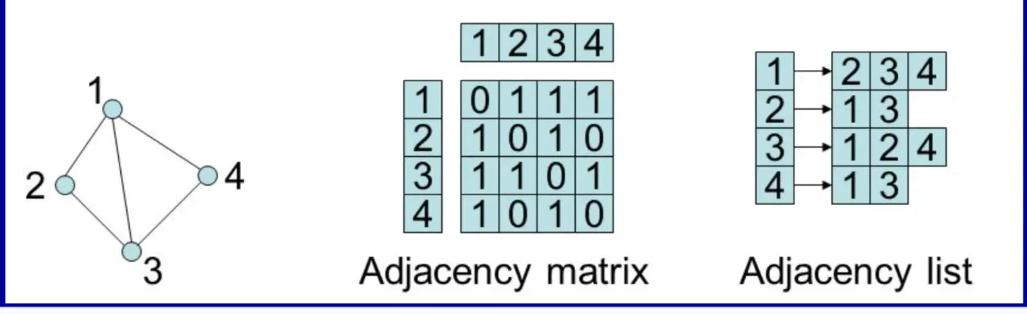
Store a numerical representation of words as tables (preferably integers)

Decision tree → which representation to use?

	Few edges (sparse)	Many edges (dense)
Few vertices	Either works; list slightly leaner	Matrix → fast lookup, small enough
Many vertices	Adjacency list → matrix wastes O(V²) on zeroes	Adjacency matrix → O(1) edge lookup matters more than space

Adding Weights

Adjacency list → store the weight alongside the neighbor (tuple, or extra data member on the edge node)
Adjacency matrix → store the weight directly in the matrix cell at the crossing

Graph Search

What are some possible ways to search a graph?
- Go all the way to the furthest point, back up to the last branch, exhaust that line too, repeat → DFS
- At each node, go one step out until all paths are exhausted, then advance another step → BFS
- Could also go randomly
- Level-order search (by distance away) → close to BFS

Breadth First Search (BFS)

Analogy → go to university and take ALL the intro courses FIRST; then advance to the next level for each
“Distance” → number of vertices in path
Visit vertices in increasing order of distance from the starting point
Use a queue to store vertices “to visit”
Not necessarily unique
Explore breadth first, then depth
May find the shortest distance to some node
Breadth First Search animation

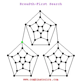
BFS finds the shortest path (in # of edges) to the solution.

VertexList bfs(const Graph& graph, Vertex startVertex) {
    VertexList result;
    // visited[v] → have we already enqueued vertex v? prevents revisiting
    vector<bool> visited(graph.size(), false);
    // queue of vertices we've discovered but haven't processed yet
    queue<Vertex> queue;
 
    // mark the start as visited and put it in the queue
    visited[startVertex] = true;
    queue.push(startVertex);
 
    while (!queue.empty()) {
        // grab the next vertex in FIFO order (closest one we haven't done yet)
        Vertex vertex = queue.front();
        queue.pop();
        result.push_back(vertex);
 
        // look at every neighbor reachable from this vertex (adjacency list)
        for (Vertex v : graph.edges_from(vertex))
            if (!visited[v]) {
                // first time seeing this neighbor → mark and enqueue
                visited[v] = true;
                queue.push(v);
            }
    }
    return result;
}

Depth First Search (DFS)

Less memory than BFS
Major example → go as deep as possible in computer science; when you don’t get a job you go to medicine; then you become a plumber
Explores depth, then neighbors
Depth in DFS isn’t necessarily the same as distance in BFS
Discover vertices before we visit
Use a stack to store nodes “to visit”
DFS order may not be unique!
Depth First Search animation

VertexList dfs(const Graph& graph, Vertex startVertex) {
    VertexList result;
    // visited[v] → have we already pushed vertex v? prevents revisiting
    vector<bool> visited(graph.size(), false);
    // stack of vertices we've discovered but haven't processed yet (LIFO)
    stack<Vertex> stk;
 
    // mark the start as visited and push it
    visited[startVertex] = true;
    stk.push(startVertex);
 
    while (!stk.empty()) {
        // grab the most recently pushed vertex (deepest one we've seen)
        Vertex vertex = stk.top();
        stk.pop();
        result.push_back(vertex);
 
        // look at every neighbor reachable from this vertex
        for (Vertex v : graph.edges_from(vertex))
            if (!visited[v]) {
                // first time seeing this neighbor → mark and push
                visited[v] = true;
                stk.push(v);
            }
    }
    return result;
}

BFS vs. DFS Tradeoffs

	BFS	DFS
Data structure	Queue (FIFO)	Stack (LIFO) — or recursion
Memory	O(branching width) — can blow up on wide graphs	O(depth) — usually much smaller
Finds shortest path?	Yes (in # of edges, unweighted graphs)	No — finds a path, not the shortest
Order of visit	Level by level out from source	Down one branch as far as possible before backtracking
Best for	Shortest-path queries, level-by-level work	Cycle detection, topo sort, exhaustive exploration

Iterative Deepening DFS

NOT MUCH MEMORY and SHORTEST SOLUTION
- (trade-off → redoing work)
Depth-limited version of DFS, run repeatedly with increasing depth limits, until solution is found
Optimal like BFS, but uses much less memory
Iterative Deepening

Topological Sorting

Operates on a Directed Acyclic Graph (DAG)
Produces a sorted order where all of a node’s predecessors appear before the node itself
Useful when computing some property on a graph that requires computations of predecessors
E.g. scheduling tasks that depend on other tasks
- Tasks → eat food, cook food, mix food, wash food, buy food
- Dependencies → buy → wash → mix → cook → eat
- Topological order → [buy, wash, mix, cook, eat]
- Pre-ordering (when first discovered): buy(1), wash(2), mix(3), cook(4), eat(5)
- Post-ordering (when finished): eat(1), cook(2), mix(3), wash(4), buy(5) → reverse post-order gives topo order
End up with levels of stuff — items on the same level can be done in parallel; everything in a level above requires the level under it
- Coursework prereqs are the classic example

Topological Sort Algorithm (Kahn’s algorithm, in-degree based):

vector<int> topologicalSort(const vector<vector<int>>& graph) {   // adjacency list
    vector<int> inDegree(graph.size(), 0);
    vector<int> result;
    queue<int> q;
 
    // Calculate in-degree for each vertex
    for (const auto& edges : graph)
        for (int vertex : edges)
            inDegree[vertex]++;
 
    // Enqueue vertices with in-degree 0 (no prerequisites)
    for (int i = 0; i < graph.size(); ++i)
        if (inDegree[i] == 0)
            q.push(i);
 
    while (!q.empty()) {
        int currVertex = q.front(); q.pop();
        result.push_back(currVertex);
        // Decrease in-degree of adjacent vertices; if any hit 0, they're ready
        for (int adjVertex : graph[currVertex])
            if (--inDegree[adjVertex] == 0)
                q.push(adjVertex);
    }
    return result;
}

Lecture 13: Minimum Spanning Trees (Prim’s, Kruskal’s, Disjoint Sets)

Minimum Spanning Trees (MST)

Spanning tree
- spanning → connects every vertex
- tree → acyclic (no cycle)
- Start with a connected, undirected, edge-weighted graph G
- A sub-graph with a subset of edges that connects all vertices
- |E| = |V| − 1 → edges is vertices minus one
Minimum spanning tree
- Sum total of edge weights is minimized
- Edge weights need not be distinct → MST need not be unique
Example → wiring a house with minimal cable

ACTIVITY → what are some possible approaches?

Check all possible spanning trees and select the shortest one
Pick the shortest edge first and try to grow from there
Choose the shortest path → O(N²)

MST Algorithms

Two common ones
- Prim’s
- Kruskal’s
Both are greedy algorithms → take the best choice at each opportunity
Difference is in how the next edge is selected

Prim’s Algorithm

Grows a single tree
Start with a single vertex, called the root
Select the minimum edge connecting (u, v) such that u is already in the spanning tree and v is not
Grow MST by adding one vertex and one edge at a time
O(|V|²) without heaps for the priority queue
O(|E| log |V|) with heaps

NEW NAME (behind me, allergies) → Josiah

Kruskal’s Algorithm

Grows a set of trees (a forest that eventually merges)
Start with |V| single-node trees
Identify the next cheapest edge
If the edge links two different trees → add it to the MST
- Adding an edge joins two trees into one
Minimum spanning tree animation
O(|E| log |V|) → much better in practice

Disjoint Set

Disjoint-set
- Needed for Kruskal’s MST algorithm
- Answers → are two vertices in the same tree (same set)?
ACTIVITY → how can we implement union/find for disjoint sets?
Three operations → make_set(), union(u, v), find(v)
- make_set → make a node whose parent points at itself; do this for every vertex → n disjoint sets to start
- find(v) → who is your representative node? Returns the address of the last node in the chain — should be one step away, since WE ALL POINT TO ONE
- union(u, v) → joins two sets together (collapse them so both point to one leader)

Disjoint-Set Data Structure

AKA
- union-find data structure, or
- merge-find set
Wikipedia → Disjoint-set data structure

Union-Find Disjoint Sets

“Disjoint set” means the sets share no elements
Create a mapping from vertices (ints) to nodes
- make_set(v) → easy with a vector inside a class
- For N items → N linked lists of length 1
- Set the parent of each node to point to itself
find(v) → returns the last node in the list
- The node’s address acts as the set’s identity
union(u, v) → joins two disjoint sets together
- find(u).parent = find(v)

Drawback → linked lists can grow long for large sets!

Performance improvements (apply in order):

Union by size/rank → always have the shorter list point to the root of the longer list
Path compression → every time we do union() or find(), set the parent to the result returned by find(v) so future lookups are O(1)

Union-Find Disjoint Sets — Resources

Kruskal’s Algorithm in C++

// Edge with two endpoints and a weight
struct Edge {
    int u, v;
    int weight;
};
 
vector<Edge> kruskalMST(int numVertices, vector<Edge>& edges) {
    vector<Edge> mst;
 
    // 1. Sort edges by weight, ascending → cheapest first
    sort(edges.begin(), edges.end(),
         [](const Edge& a, const Edge& b) { return a.weight < b.weight; });
 
    // 2. Start with each vertex in its own set
    DisjointSet ds(numVertices);
 
    // 3. Walk edges cheapest → most expensive
    for (const Edge& e : edges) {
        // If u and v are already connected, adding this edge would form a cycle → skip
        if (ds.find(e.u) != ds.find(e.v)) {
            mst.push_back(e);          // edge links two different trees → take it
            ds.unionSets(e.u, e.v);    // merge the two trees into one
            if (mst.size() == numVertices - 1) break;  // MST has |V| − 1 edges, done
        }
    }
    return mst;
}

Kruskal Example

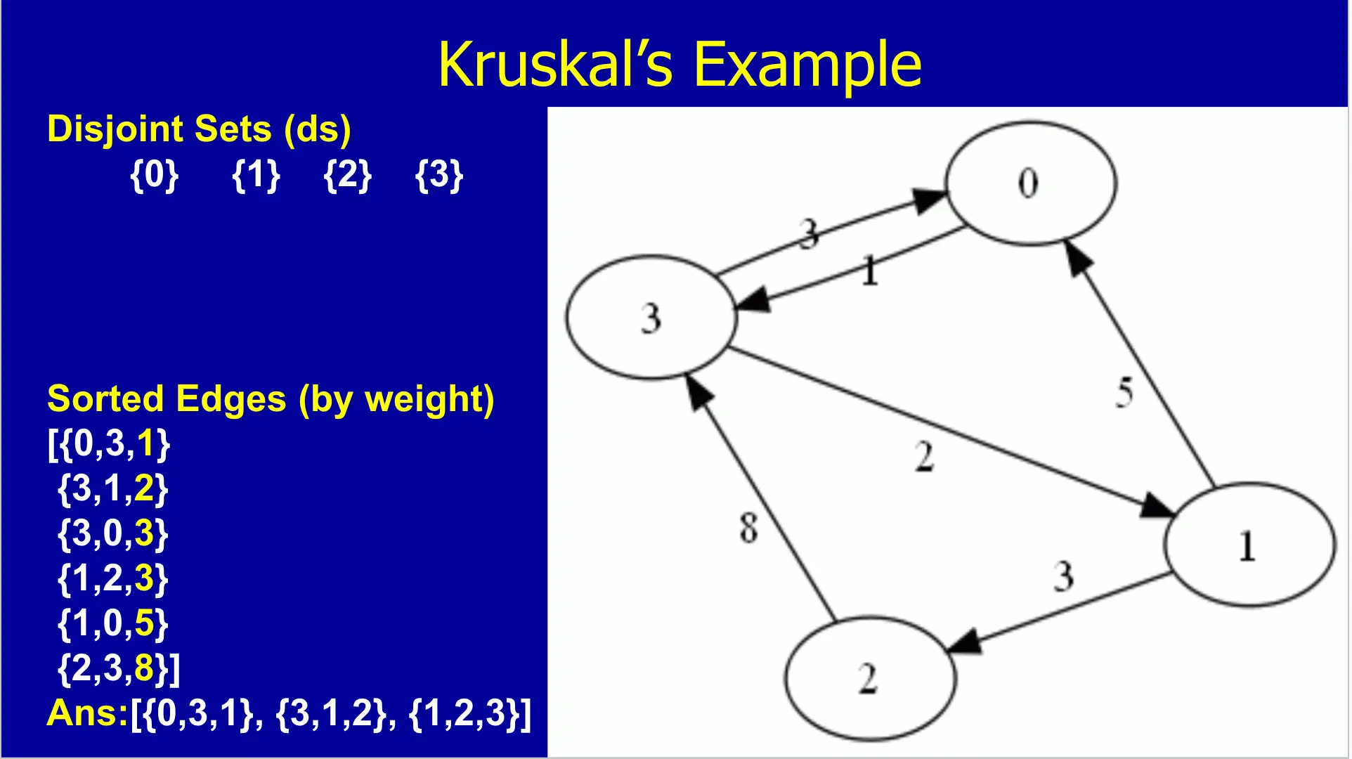
Lecture 14: Single-Source Shortest Path (Dijkstra’s, Word Ladder)

More Graph Problems

Unweighted graphs → BFS / DFS for traversal and reachability
Directed Acyclic Graphs (DAGs) → topological sort to order tasks by dependency
Weighted graphs
- Minimum spanning tree → cheapest set of edges connecting every vertex (covered in Lecture 13)
- Single-source shortest path → cheapest path from one start vertex to every other
- Traveling salesman problem → shortest tour that visits every vertex exactly once (NP-hard)
Network flow
- Maximum flow → most “stuff” you can push from a source to a sink under edge capacities
Heuristic → rule-of-thumb to narrow the search space
- “Control the center” is a heuristic for picking a good opening move in chess

Single-Source Shortest Path (SSSP)

Given
- A graph G = (V, E)
- A single starting vertex s
Find the lowest-cost path from s to every other vertex
For unweighted graphs → BFS (every edge treated as cost 1)
For weighted graphs → several choices
- Dijkstra’s algorithm → only positive weights
- Bellman-Ford → handles negative weights too, O(|V|·|E|)
- A* → heuristic-guided; needs an upper-bound distance estimate to the goal
  - GPS routing uses A* with straight-line Euclidean distance as the heuristic
  - An example of best-first search

Applications

Maze games
Street routing (driving directions)
Trip planning
Network packet routing
Robots navigating around obstacles
Dijkstra animation
Example 1 · Example 2

Naive Brute-Force Shortest Path

Enumerate every simple path from s to t and take the minimum
Explodes combinatorially → useless beyond toy sizes, but shows what “correct” looks like

// Try every simple path from s to t via DFS, track the smallest total weight
// graph[u] = list of (neighbor, weight) pairs
int bruteForceSSSP(const vector<vector<pair<int,int>>>& graph, int s, int t) {
    int n = graph.size();
    vector<bool> visited(n, false);
    int best = INT_MAX;
 
    function<void(int, int)> dfs = [&](int u, int cost) {
        if (u == t) { best = min(best, cost); return; }
        visited[u] = true;
        for (auto [v, w] : graph[u])
            if (!visited[v]) dfs(v, cost + w);
        visited[u] = false;  // backtrack so other paths can still go through v
    };
 
    dfs(s, 0);
    return best;
}

Dijkstra’s Algorithm

A greedy algorithm, published by Edsger Dijkstra in 1959
Maintain distance estimates to every neighbor of s
Repeatedly pull the unvisited vertex with the shortest known distance, add it to the visited set, then relax (update) the distances of its neighbors
Does not work on graphs with negative edge weights
O((|E| + |V|) log |V|) with a binary heap as the priority queue

// Dijkstra's SSSP on a non-negative weighted graph
// graph[u] = list of (neighbor, weight) pairs
// Returns shortest distance from s to every vertex
vector<int> dijkstra(const vector<vector<pair<int,int>>>& graph, int s) {
    int n = graph.size();
    vector<int> dist(n, INT_MAX);
    dist[s] = 0;
 
    // Min-heap of (distance_so_far, vertex)
    priority_queue<pair<int,int>, vector<pair<int,int>>, greater<>> pq;
    pq.push({0, s});
 
    while (!pq.empty()) {
        auto [d, u] = pq.top(); pq.pop();
        if (d > dist[u]) continue;  // stale entry — already found a shorter path to u
 
        // Relax each outgoing edge of u
        for (auto [v, w] : graph[u]) {
            if (dist[u] + w < dist[v]) {
                dist[v] = dist[u] + w;
                pq.push({dist[v], v});
            }
        }
    }
    return dist;
}

Walkthrough 1 · Walkthrough 2
HW9 → read the same graphs from HW8, but compute Dijkstra’s
- Output the path and total cost to each vertex from the start
- Be able to answer questions like → “what is the cost from start to vertex K?”

Word Ladder Problem

LeetCode (medium/hard) · GeeksforGeeks
A transformation sequence from beginWord to endWord using a dictionary wordList is a sequence
- beginWord → s₁ → s₂ → ... → sₖ → endWord
- such that
  - every adjacent pair of words differs by a single letter (or one insert/delete)
  - every sᵢ (for 1 ≤ i ≤ k) is in wordList
  - beginWord need not be in wordList, but endWord must be
The problem → find the shortest such transformation sequence

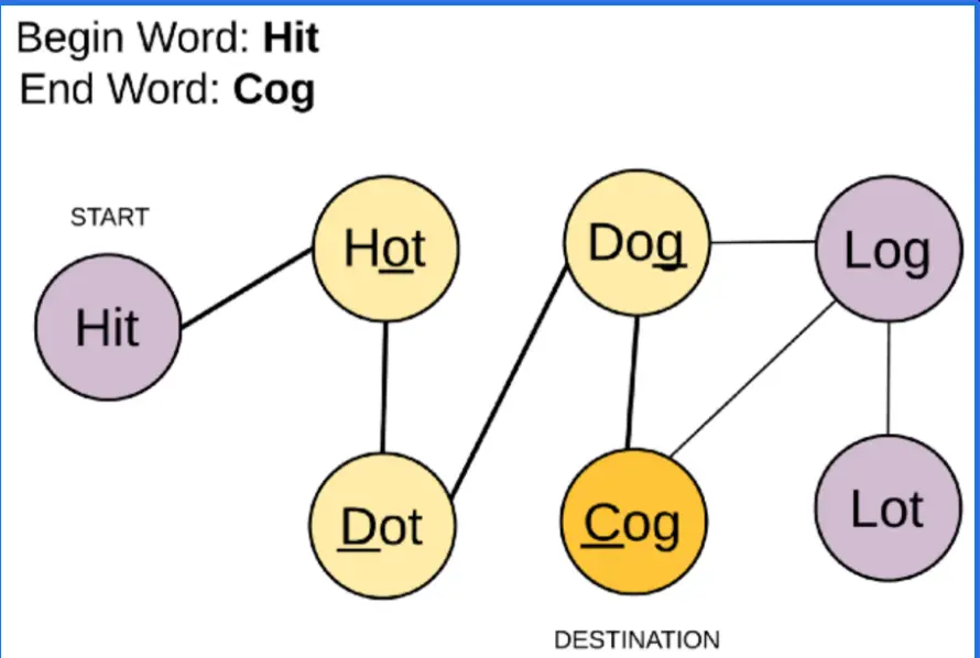
Word Ladder Videos

Solution Sketch

A solution uses breadth-first search
- Queue holds stacks (each stack is a candidate ladder so far), implemented with vector
- Maintain a set of words already used so we don’t revisit and loop forever
BFS guarantees the first time we pop endWord off the queue, we’ve found a shortest ladder

Course Review

Course Topics

Time analysis and time complexity
Lists: Unordered, Ordered, Sorted
Stacks & Queues
Hashing and Hash Tables
Binary Search Trees
Priority Queues (Binary Heaps)
Sorting & Searching
Graph representation
Graph traversals
Graph algorithms

Analysis

T(N) → running time in instructions, worst case
- Accessing during a for loop counts as + 1
- For if statements we take the worst-case branch
- A return costs 1 + cost of the expression
Time complexity in Big-O notation
Measured (empirical) time of algorithms
- Using Timer.h
Interpreting graphs of functions → what are we actually measuring?
Thinking about our testing data → and the unusual measurements we may get

Lists: Unordered, Ordered, Sorted

Unordered
- Must use linear search
- Doesn’t matter where you add/remove → so we choose the spot that’s O(1)
Ordered
- Like class string
Sorted
- Forces copy-up / copy-down on insert/remove
- Can use binary search to find

Stacks & Queues

Stack interface (LIFO) → push(), pop(), top(), isEmpty(), isFull()
Queue interface (FIFO) → enq(), deq(), front(), isEmpty(), isFull()
Implementations are all constant time:
- Linked list: stack, queue
- Array: stack, queue

Hashing & Hash Tables

Tables → key/value pairs
Critical decisions:
- Choose a good hash function
  - URLs are hard and most of the time break the hash function
- Choose a table of good size
- How to handle collisions
  - Separate chaining
  - Open addressing (e.g. linear probing)
insert, find, remove can be O(1)

Binary Search Trees

insert, find, remove can be O(log N)
Traversals: pre-order, in-order, post-order
Degenerates to O(N) when keys are nearly sorted
Fixed with self-balancing trees → AVL, red-black, WAVL, crumple

Sorting & Searching

O(N²) sorts
- Insertion sort
- Selection sort
- Bubble sort
O(N log N) sorts
- Quick sort
- Heap sort
- Merge sort
Sorting visualization videos:

Graph Representation

Representation:
- Adjacency list
- Adjacency matrix
What are the trade-offs?
What did you do for edges_from in HW8?
- VertexList Graph::edges_from(vertex vertex) const

Graph Traversals

Depth-first (DFS)
- Can get stuck going down a cycle forever → needs a visited set
Breadth-first (BFS)
- Finds the shortest path to the solution (fewest edges)
Iterative deepening DFS (IDDFS)
- ELI5: run DFS but only let it go K levels deep, throw it away, then run it again allowing K+1 levels, then K+2, … → a for loop over the depth limit K that keeps re-running a depth-limited DFS until the goal shows up
- Gets BFS’s shortest-path guarantee (finds the shallowest goal first) with DFS’s small O(depth) memory
- Yes it re-explores the shallow nodes every round, but that’s cheap → almost all the nodes live at the deepest level anyway
Best-first search

Graph Algorithms

Topological sort
Minimum spanning tree: Kruskal’s, Prim’s
- Kruskal’s → be able to derive
Shortest path: Dijkstra’s, Bellman-Ford, A*

Ivan's CS Notes

Explorer

ICS_46